A key concept in RL is learning the value function with bootstrapping. But there are several objectives that all make use of bootstrapping, all of which differ in subtle but important ways. For instance, we have Bellman Error Minimization, TD Learning, Partially Fitted Value Iteration, not to mention Mean Squared Projected Bellman Error, oh my…

Making things more confusing, standard treatment of these algorithms (e.g. from Sutton and Barto) uses linear value function estimation. In that case, the span of the tangent line of the value estimate is the same as the hypothesis class itself. As we shall see, when the value estimate is not linear in its parameters, intuitions from linear RL break down.

In this post, I demonstrate the behavior of the following non-linear value function learning methods on the spiral MDP:

• Fitted Value Iteration (FVI)
• TD Learning
• Bellman Error Minimization
• Projected Bellman Error Minimization
• Monte Carlo / Supervised Value Learning

The Spiral MDP

Tsitsiklis and Van Roy devised a counterexample to demonstrate that TD learning fails on-policy with non-linear function approximation. As we will see, the spiral MDP also breaks fitted value iteration.

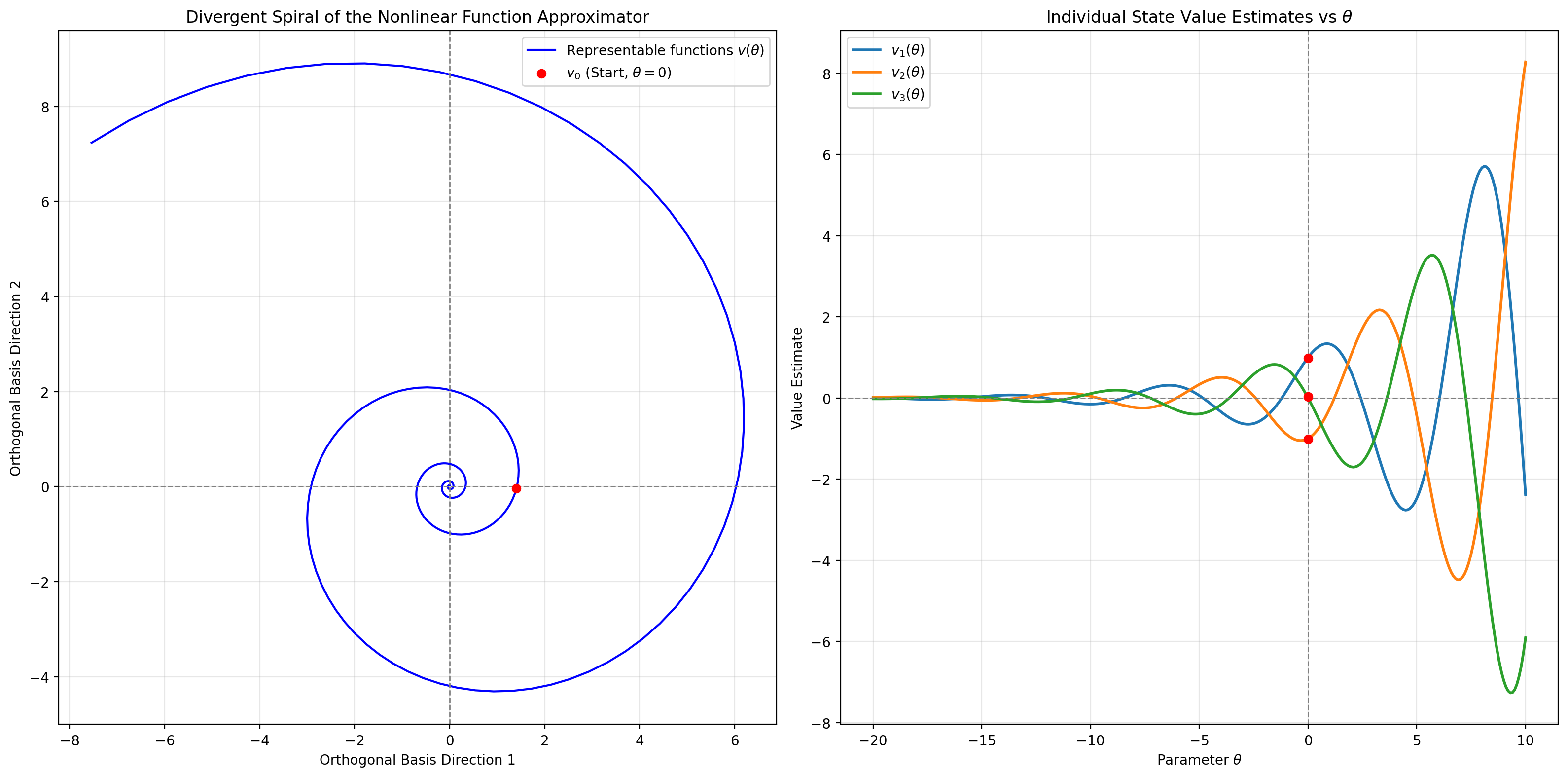
The problem is a Markov Reward Process (MRP) and value function estimator. The MRP has three states, thus the value function estimate, called \(v_\theta\), outputs a three-dimensional vector that depends on a single parameter \(\theta\). The reward is zero everywhere, meaning the true value is \(V^\pi = \mathbf{0}\). The magnitude of the estimate \(v_\theta\) approaches zero as \(\theta \rightarrow -\infty\).

The value function, and its estimate are in three dimensions. However, \(v_\theta\) will always live in a two-dimensional subspace. We visualize that subspace in Figure 1. The spiral shows our function class – all possible values of \(v_\theta\) (projected to the 2-D subspace). The sinusoidal curves show the value function as the \(\theta\) changes - with each color representing a different state value.

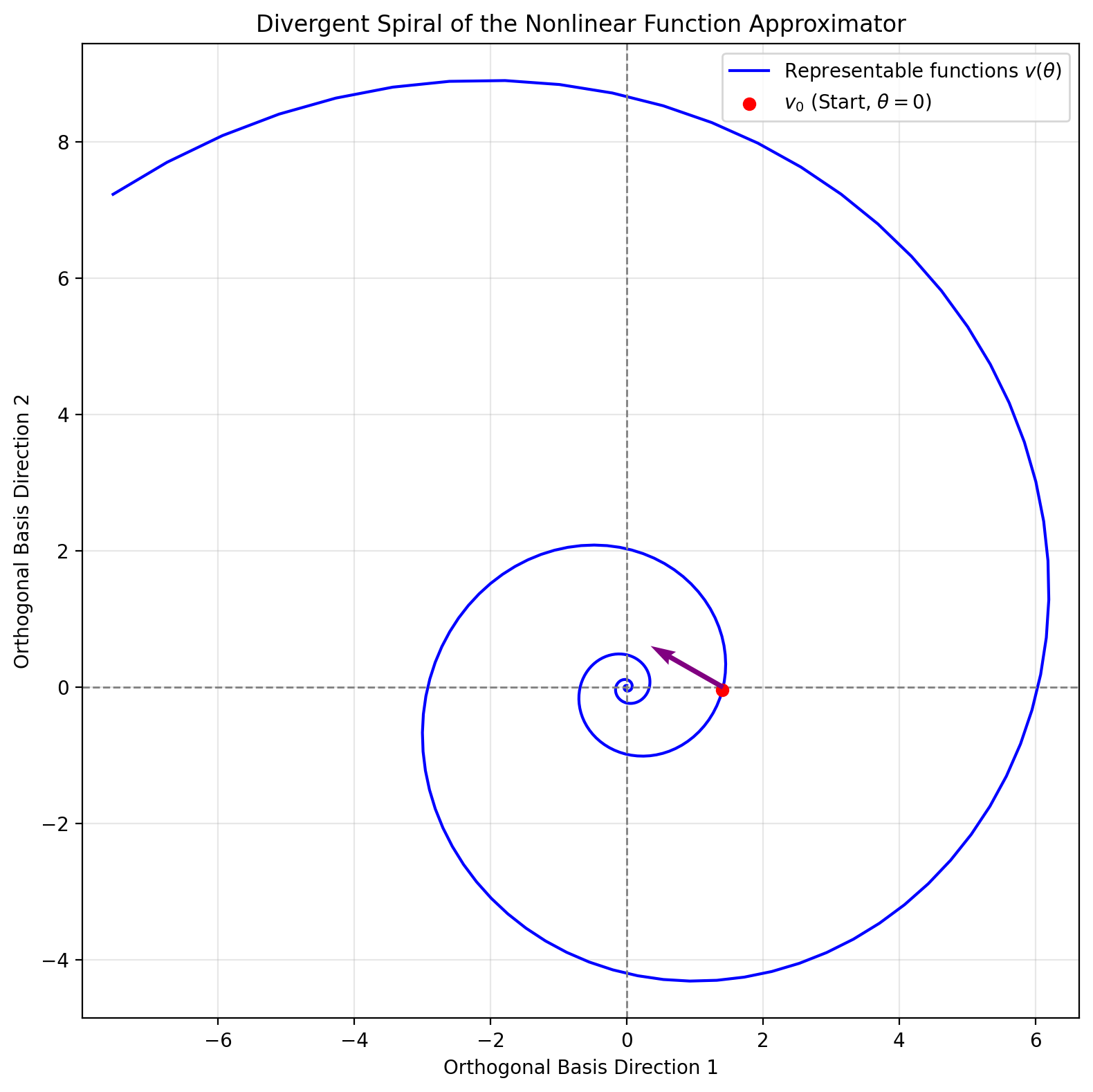
Figure 1: The Spiral MDP.

What’s nasty about this MRP – at least from the point of view of TD learning and friends – is that the Bellman Operator points towards the true value center, but when fitting it as a stationary target (like most bootstrapping methods), \(v_\theta\) fits the Bellman Estimate of the value, yet it diverges from \(V^\pi\).

A few technical details. First, the Bellman Operator is closed in this 2D space. For those who are curious why: \(\mathbf{1} =(1,1,1)^\intercal\) is a left eigenvector of \(P\) with eigenvalue 1. This implies that for any vector \(v\) orthogonal to \(\mathbf{1}\), \(Pv\) remains orthogonal to \(\mathbf{1}\), since \(\mathbf{1}^\intercal P v = \mathbf{1}^\intercal v = 0\).

Technical detail 2: The state-visitation distribution in the spiral MDP is exactly one third times the identity. Thus the on-policy weighted distance reduces to a constant scalar times the Euclidean distance. Technically, all inner products should be weighted by the on-policy distribution (stored in the matrix \(D\) in my earlier posts), but because \(D = \frac{1}{3}I\), I ignore it in this post. See the final section of the original paper for the description of the MRP.

Figure 2: Bellman Operator.

Algorithm 1: (Partially) Fitted Value Iteration (FVI)

(Partially) Fitted Value Iteration (FVI) is the most common value learning algorithm in deep RL. For example, DQN and PPO both perform FVI. Generally, FVI is thought of as a batch algorithm. It repeatedly fits the Bellman Operator. In expectation, it works as follows:

Algorithm: FVI
Repeat:
0. Initialize Target Network u <- v.
1. Estimate Tu = R + γPu.
2. Compute v by minimizing the length of Tu-v.

The distinction between batch FVI and PFVI lies entirely in the final step, when a new value estimate is obtained as \(v_\theta \gets \operatorname{argmin}_{v_\theta} \|Tu - v_\theta\|^2\). In classic linear FVI, the best fit for \(\theta\) can be obtained using least squares regression.

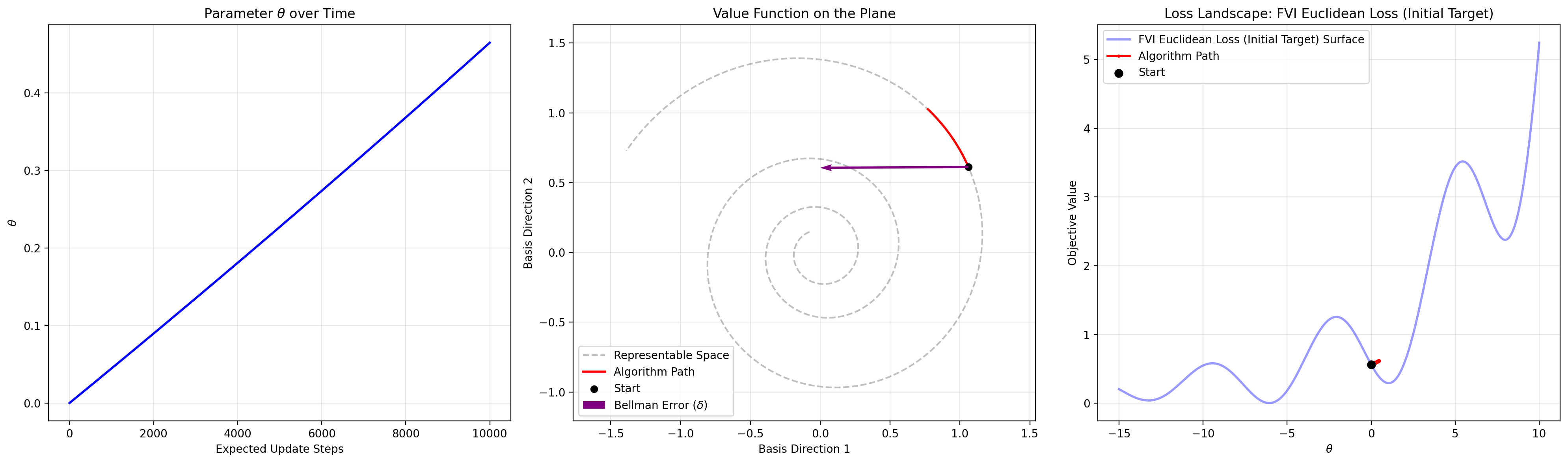
Deep variants perform gradient descent on \(\theta\). But for how many gradient updates? If we fit \(\theta\) for just one step of gradient descent, we get TD learning. If we run gradient descent until convergence, we get full batch FVI. The crux of the problem is that gradient descent doesn’t give us a global minimum. And the local optimum obtained is unfortunately worse than what we started with.

I run FVI on the spiral problem, with 200 gradient steps per Bellman update. The learning dynamics shown are in Figure 3. The left panel shows the parameter value with each update – notice that it is diverging away from the best estimate \(\theta^* = -\infty\). The middle panel shows the trajectory on the spiral. The trajectory appears to be going in the wrong direction, despite a better fit being available in the function class. How can this be? As the right panel shows: the loss landscape is non-convex. The global minimum estimator appears to be far to the right, around \(\theta=-5\). But there is a different local minimum in the other direction. Because the loss landscape is non-convex, each round of FVI gets further away from \(Tv\).

Figure 3: Learning Dynamics of FVI.

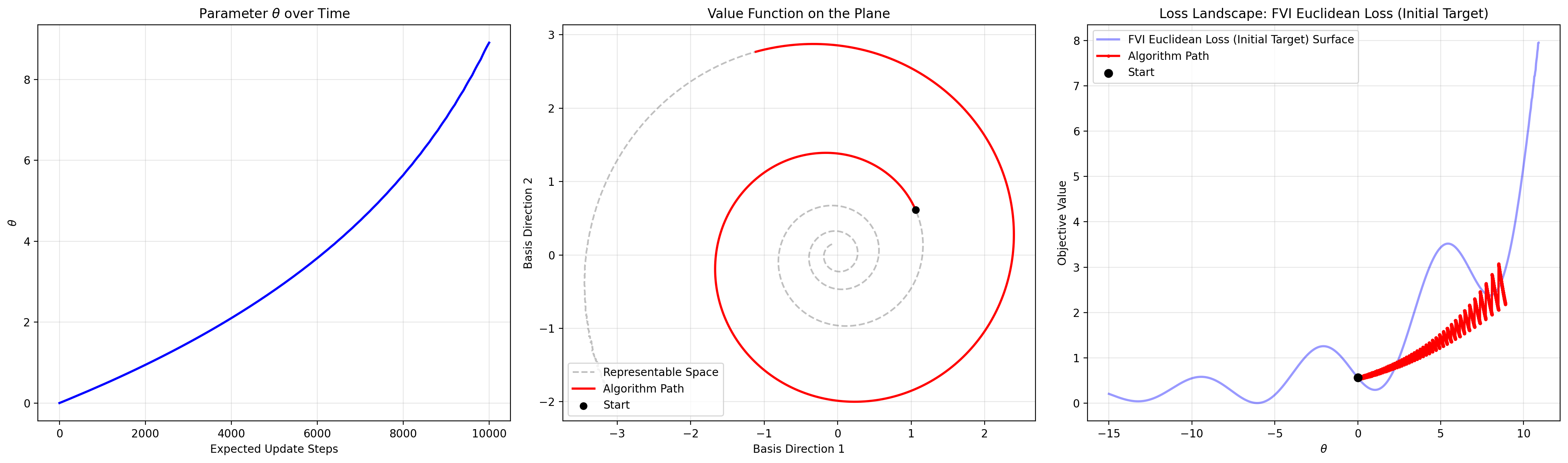
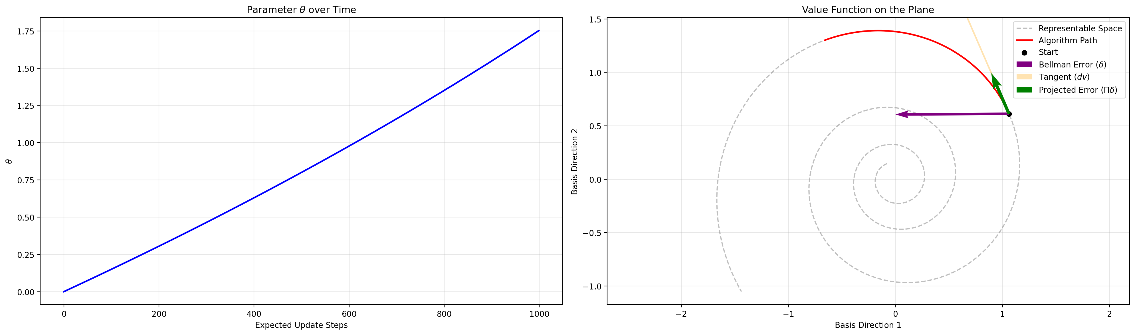
Because our \(v_\theta\) is non-convex, fitting the Bellman operator can lead to a worse value estimate, breaking the contraction argument for why standard exact value iteration converges. In short, the “fitted” component of FVI breaks the guarantee of value iteration. Figure 4 shows a longer run. Note that the parameters traverse the fixed loss landscape, since the loss changes with each application of \(T\) (but I only show the first loss).

Figure 4: Longer Run of FVI.

Algorithm 2: TD Learning

Tsitsiklis and Van Roy’s original 1997 paper analyzed TD learning. As mentioned above, TD learning takes a single gradient step to fit the Bellman Operator before updating the value function. A single gradient step is a locally linear approximation to the true optimal direction. As such, each step of TD learning can be understood as taking a small step towards the projection of \(Tv_\theta\) onto the space orthogonal to the tangent line of \(v_\theta\).

Figure 5 shows the dynamics of TD learning. Again, a single application of the Bellman Operator to the starting value estimate is shown in purple. The green line shows the projection of \(Tv_\theta\) onto the span of \(\nabla_\theta v\) (a length 3 vector with entries \(\frac{dv}{d\theta}(s_i)\) for each state). Notice that this line points away from the center due to the direction of the spiral and angle of \(T\).

Figure 5: TD Learning.

def td_update(θ, v, dv, α):
    δ = T(v) - v
    θ = θ + α * dv.T @ δ
    return θ

Note that in the linear case, the span of the tangent line is the space of representable functions. In this case, FVI and TD learning have the same fixed point.

Algorithm 3: Bellman Error Minimization (BEM)

Bellman Error Minimization (Baird, L. (1995)) solves \(\min_{\theta} \|Tv_\theta - v_\theta\|_2^2\). This looks a lot like TD learning and FVI. The key difference is that BEM differentiates both \(v_\theta\) AND \(T v_\theta\) with respect to \(\theta\). Whereas TD learning and FVI fix \(T v_\theta\) (e.g. with a target network).

The presence of \(\nabla_\theta T v_\theta\) means that BEM techniques must incorporate information about how \(Tv\) changes with \(v\). More precisely, BEM methods must estimate \(P \nabla_\theta v_\theta\) – the expected value of the gradient one step into the future – as well as \(\delta\), and take their product. Since the expectation of a product does not equal the product of expectations, a naive sample-based update requires two independent transitions from the same state (the double sampling issue). However, just as in GTD methods, one can circumvent double sampling by introducing an auxiliary weight vector to estimate the expected future gradient product without requiring two next-state samples. In our experiments on the spiral problem, we can compute all terms in the gradient exactly.

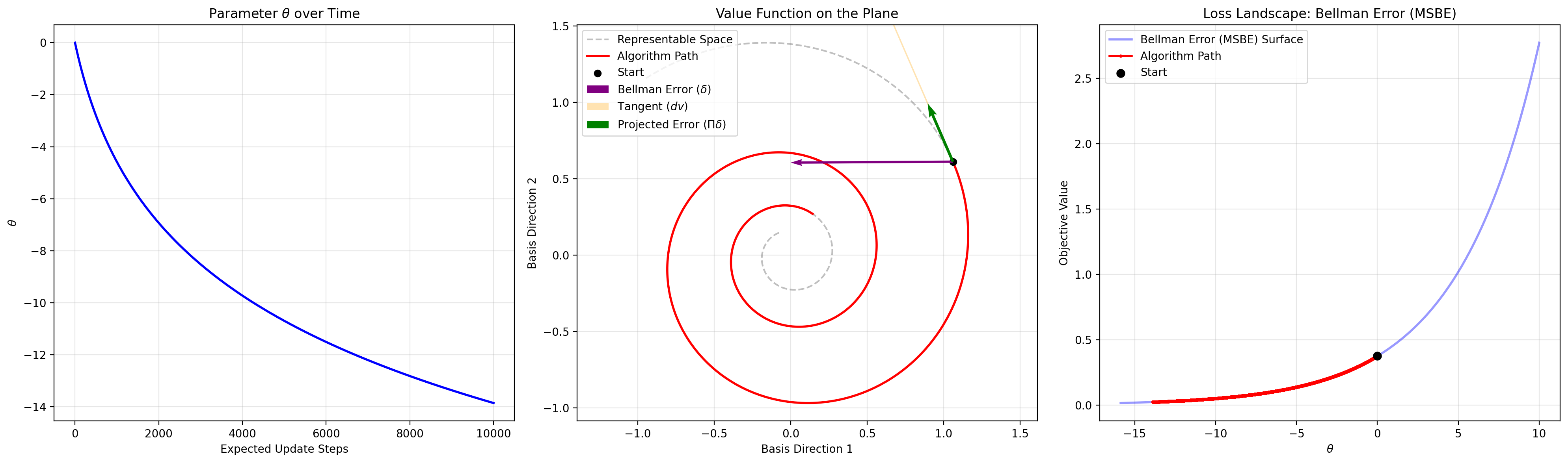
Results are shown in Figure 6. Note that BEM succeeds on this problem.

Figure 6: Bellman Error Minimization.

Algorithm 4: Mean Squared Projected Bellman Error (MSPBE)

The MSPBE is the length of the green vector in Figure 5. Letting \(\Pi_\theta\) be the linear projection onto the span of \(\nabla_\theta v\), we have:

Since we have just one parameter, \(\Pi_\theta\) is the \(3\times3\) matrix:

Plugging this in, we the squared TD learning update, divided by the squared length of the tangent vector \(\|\nabla_\theta v\|^2\):

There are numerous issues minimizing this quantity. For one, the gradient of the MSPBE contains the product of value network Hessians. Secondly, it once again requires estimating \(P \nabla_\theta v_\theta\) – in other words, it must know how $v_\theta$ changes as a local function of \(\theta\). This also requires addressing the double sampling issue. Methods that minimize the MSPBE avoid double sampling by training an estimator to predict the Bellman error.

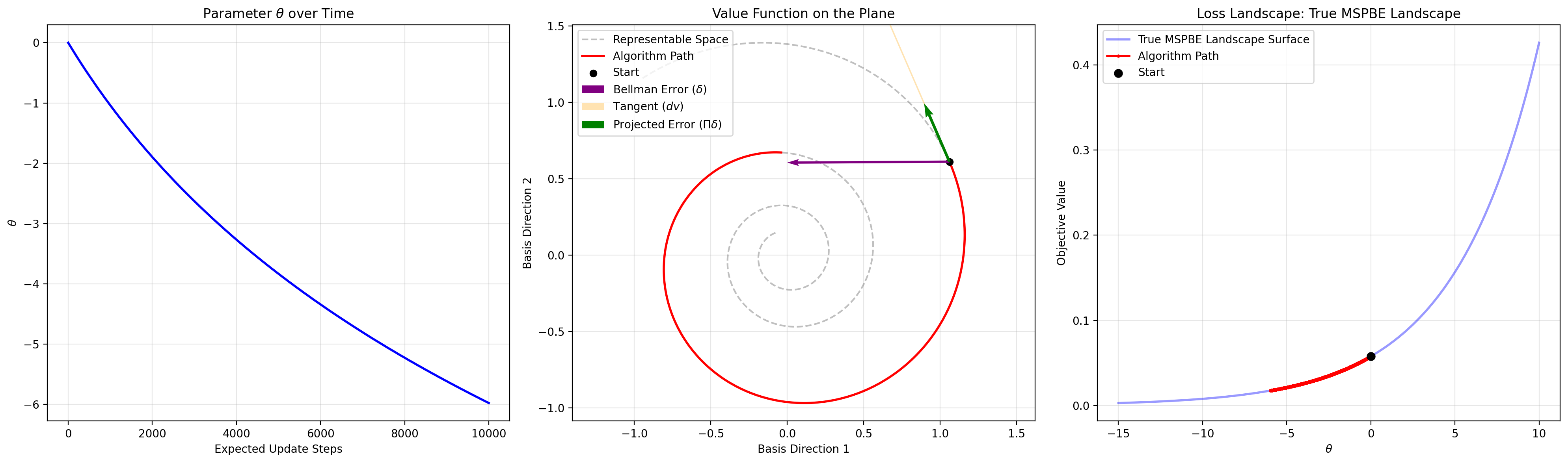
For our toy problem, we can compute the gradient of the MSPBE exactly - and find that it works! At each step, it can be thought of as changing \(\theta\), re-applying the Bellman operator, and measuring the length of the green line. The right panel shows the true MSPBE - or the length of the green vector - as learning progresses.

Figure 7: MSPBE Minimization.

Algorithm 5: Monte Carlo

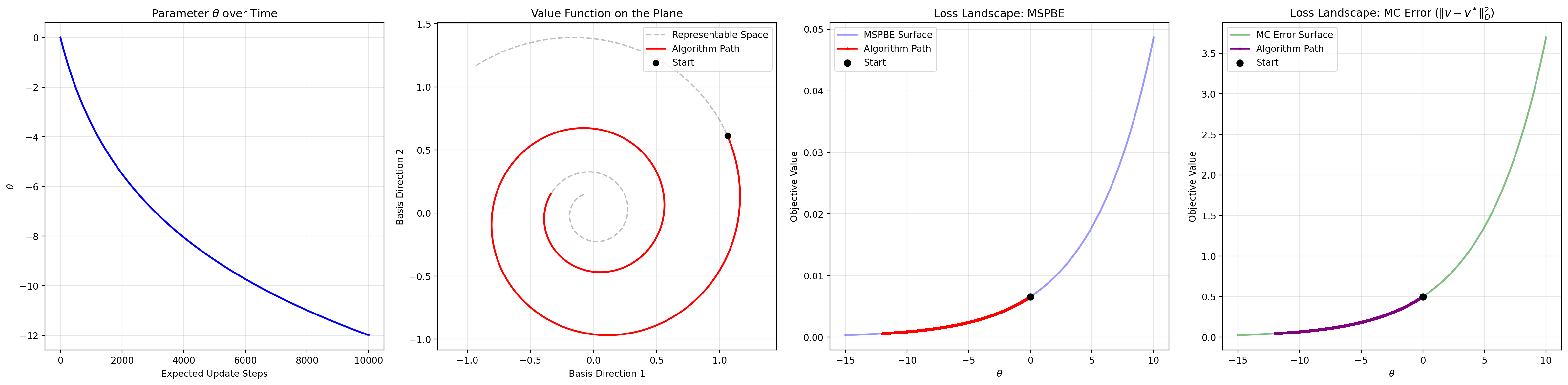
Removing all sampling noise, Monte Carlo value learning is just supervised learning of the center of the circle. Does this suffer from a highly non-convex landscape like FVI?

It does not. As \(\theta\) decreases, the error monotonically decreases as well, leading to a convex loss landscape. Note that its loss, shown in the fourth panel of Figure 8, has quite a similar shape to the MSPBE error, which is shown in the third panel.

Figure 8: Monte Carlo / Value Error Minimization.

Summary

In short, all one-step methods either fail (TD and FVI), or face the double sampling issue (BEM and MSPBE minimization). In our experiments, we take advantage of access to the true transition matrix and reward function to bypass the double sampling issue. Additionally, we get strong performance from multi-step methods like MC / VEM, due to the absence of sampling variance.

Refresher

The last post derived theoretical conditions for when TD learning fits the value function. Earlier theoretical results (Tang and Munos (2023)), found that if the Markov Chain is reversible ($\mu_i P_{ij} = \mu_j P_{ji}$), then TD-Learning is the exact same as gradient descent on a symmetrized value error. Let our estimate be $v_\theta$ and the value error vector be $e=V-v_\theta$. Finally, recall the definition of the key matrix $A=D(I-\gamma P)$. Then, the value error is the following:

Where $S = \frac{1}{2}(A + A^\top)$, and the second line follows from the fact that $E$ is quadratic, meaning only the symmetric part of $A$ matters. Since $E$ is a (weighted) norm, it can only be zero if $e=0$. This implies the typical value error $\overline{VE}^2 = e^\top D e^\top$ and $E$ have the same minimum.

TD Learning

TD learning is based on bootstrapping. Its update is proportional to:

Next, I show that $Ae = D \delta$, giving us the form:

Proof that $Ae = D \delta$.

The takeaway is that the update $\theta$ due to TD learning is proportional to $Ae \nabla v_\theta$. Also, note that $A$ is positive semi-definite since the bellman operator $T$ is a contraction on $| \cdot |_D$.¹.

Gradient Descent on E

This is almost the same as the direction followed by direct gradient descent on $E$, which follows the negative gradient of $E$:

Tang and Munos used the near equivalence of these two expressions to show that TD learning is the same as gradient descent on $E$ exactly when $S = A$ (the MDP is reversible).

Symmetrized TD Learning

However, in general, $A$ is not symmetric, and $A = S + K$, with skew-symmetric component $K \doteq \frac{1}{2}(A-A^\top)$. This means that the skew-symmetric component is what can derail TD learning. The natural question is if we can remove the skew-symmetric component. Then, the TD learning update would take a step in the direction of $\nabla_\theta E$. We can rewrite $Se$ as $S(I-\gamma P)^{-1} \delta$. This yields an update of the following form, weighting the TD error by $S(I-\gamma P)^{-1}$ that will minimize $E$.

Whirlpool Experiments

To test this symmetrized TD learning, I compare to exact TD learning. Exact TD learning makes applies the expected update due to TD, rather than constructing the an unbiased estimate from samples. This removes the noise in TD learning. Notice it doesn’t depend on a sampled batch: instead it computes $\delta$ for all states, and then weights it by $\mu$ in the final loss.

def td_loss(params):
	v = network.apply(params, ALL_STATES) # length N vector
	TD_targets = R_π + λ * P_π @ v
	td_errors = v - stop_gradient(TD_targets)
	loss = 0.5 * jnp.sum(mu * (td_errors ** 2))
return loss

For all experiments, I train a convolutional network to evaluate a fixed policy. I use a fixed policy due to training PPO to near convergence. The I also train with exact Monte Carlo (i.e. gradient descent on $e^\top D e$), removing the variance due to noisy estimates of $V$ and noisy gradient estimates. Perhaps unsurprisingly, I find the symmetrized obtains much better value error with a neural network compared to TD learning. More suprisingly, I find it has better value erro than Monte Carlo. In the following experiment, I train a policy to near convergence with PPO.

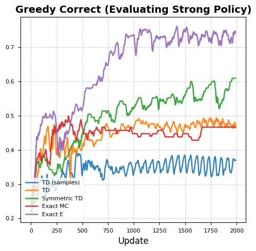
Symmetric TD found a significantly stronger policy than exact MC (regression on $V$) or exact TD.

Figure 1: Exact Algorithms performing policy evaluation of a strong policy on Four Rooms.

Surprisingly, gradient descent on $E$ found the strongest policy, suggesting there is something useful about weighting errors by $S$…

Whirlpool Environment

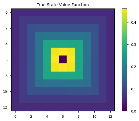
To “stump” TD, I created a more asymetric environment: a whirlpool with a reward in the center. The start state is a random state in the outer ring, and the transition function pushes the agent clockwise 90% of the time, with the agents intended action succeeding 10% of the time. The value function is the following (note the reward is given on the transition into the center state, following the standard Gym API, leading to the terminal state having zero value.)

Figure 2: Value of the whirlpool MDP. Note it is radially symmetric.

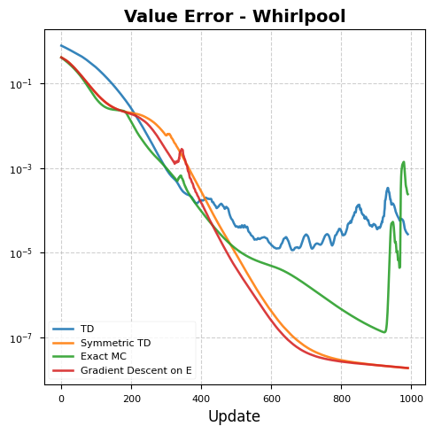
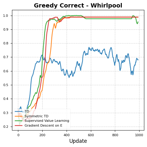
On this environment, TD was much weaker than the other methods, while gradient descent on $E$ and symmetric TD were the strongest.

Figure 3: Value Error on of the whirlpool MDP for exact methods (lower is better).

Figure 4: Greedy Policy prediction accuracy on of the whirlpool MDP for exact methods (higher is better).

Practical issues

Symmetric TD uses $(I-\gamma P)^{-1}$, essentially requiring solving the Bellman equation.

Penalizing Skew-Symmetric Portion

A related idea is as follows: subtract $Ke \nabla V$ from the TD update. This is because the difference between the TD update $(Ae \nabla v)$ and gradient of $E$ $(Se \nabla v)$ is exactly $Ke$:

This implies that $\dot{\theta} - Ke \nabla = \nabla_\theta E$. To make the TD update gradient descent on $E$, simply add $Ke \nabla v$ to the $TD$ update. However, this too requires a value oracle to get $e$, or Monte Carlo to estimate it, removing the advantage of TD learning.

(This is a follow-up to my previous post Will Deep TD Learning Result in Quality Representations?)

Deep temporal difference learning is the primary method for estimating the value function in reinforcement learning. The goal of TD learning is to minimize the average squared value error, averaged over a state distribution \(\mu\):

where \(V\) is the true value function, \(v\) is estimate, and \(D = \text{diag}[\mu]\). The value estimate, obtained from a neural network, is the dot product of the state-features and value weights: \(v(s) = \phi(s)^\intercal w\). Since the value is not directly observable, TD learning uses bootstrapping: fitting the value network towards a target based on its own predictions.

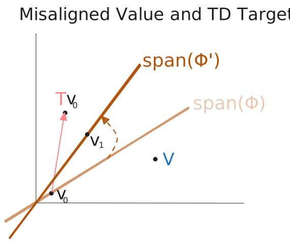
In the last post, I provided a geometric intuition and showed that deep TD learning can adjust the features in the wrong direction – raising the inherent value error \(VE\) for the best weights. This happened when the TD target and true value function are on opposite sides of the feature space, which I call misalignment. An example is pictured below.

Figure 1: An example where misalignment of the bellman target Tv and true value function V hurts the features.

Is misalignment a problem in practice? For evaluating the random policy on Four Rooms, I found it was not. But does it become an issue in challenging domains like math or robotics?

The literature has explored how deep TD learning will adjust the features. [Tang and Munos 2023] showed that, under the property that the MDP is reversible (\(D P = P^\top D\)), the TD learning update happens to perform gradient descent on \(V\). This sounds great, however, reversibility is extremely unlikely to hold in practice: It says that the probability transition \(Ds_1 \rightarrow s_2\) equals the probability of \(s_2 \rightarrow s_1\). Yet, on most tasks, strong policies don’t go backwards.

In this post, I extend the results of Tang and Munos 2023. Reinforcing the importance of alignment, I show that alignment is a necessary and sufficient condition for the value error to decrease. I also show that an almost reversible property is enough to guarantee alignment. Before that, I walk us through their original proof, which answers the important question of when TD learning is doing the right thing. So let’s go!

Main Result of Tang and Munos (2023)

This work considers a continuous-time variant of TD learning, described by the following system of differential equations:

The dot indicates the time derivative: (\(\dot{x}_t = \frac{dx}{dt}\) for a function \(x(t)\)). These equations describe the dynamics of TD learning when discrete algorithmic updates are brought into continuous time. For the purposes of this blog post, I’ll assume that the weights are a fixed value \(w_t = w\).

The key question is how the value error changes with each update. We analyze this in terms of the time-derivative of the value error, \(E\) (defined below).

We now define the value error. For theoretical convenience, Tang and Munos consider a loss that weights states slightly differently. They define a value error \(E\) that weights by the “key” matrix \(A = D(I-\gamma P)\):

Though it doesn’t appear in the standard value error, the key matrix is of massive importance for the stability of TD learning. The dynamics of the features can be rewritten in terms of the key matrix.

The true value function doesn’t appear directly. A key insight is that the Bellman equation implies \(DR = D(I-\gamma P) = AV\), allowing the above equation to be rewritten in terms of the true value function \(V\). This is an imporant move that is crucial to the results discussed in this post.

We’d like to understand how \(E\) changes as TD learning progressively updates the features. Essentially this boils down to comparing \(\dot{\Phi}_t\) with \(-\partial_\Phi E(\Phi, w)\). If they point in the same direction, then TD learning decreases the value error.

Theorem (Tang and Munos 2023, Theorem 3): Assume that \(A\) is symmetric (i.e. \(DP = P^\top D\)). Then, the TD learning update is the same as gradient descent on \(E\), i.e.:

The conclusion is TD learning is effectively supervised learning of the value function. Sounds great! However, the premise that \(A\) is symmetric is unlikely to hold. It occurs when the Markov chain is reversible, meaning the probability of the transition \(s_1 \rightarrow s_2\) is the same as \(s_1 \leftarrow s_2\). Still, disregarding this result because the premise is too strong would be a mistake. As we will see, the proof of this theorem ties TD learning and value error minimization together in a way that can be extended, allowing us to write down exact mathematical conditions for when deep TD learning will and won’t work.

To start, I provide the proof of this theorem. Then I’ll relax the reversibility condition to show our main result.

Proof of Tang and Munos Theorem 3: Define the error vector \(e_t \doteq \Phi_t w - V^\pi\), which is a function of \(\Phi\). The value error is then: \(E(\Phi_t) = \frac{1}{2} e_t^T A e_t\) Since \(E\) is quadratic, it can be rewritten as \(e_t^\top (A + A^\top) e_t\), retaining only the symmetric portion of \(A\) (this is discussed more in the next section). From there, we have:

Now let’s consider the change in features due to TD learning. Plugging \(e_t\) into the expression \(\dot{\Phi}_t = -\eta_\Phi \cdot A(\Phi_i w_i-V) w^\top_i\) from earlier gives the following similar formula.

Comparing these formulations shows that if \(A\) is symmetric (\(A^\top = A\)), then TD learning gives the same feature update as gradient descent on \(E\).

New Result: When exactly do we have alignment?

For the TD learning update to be beneficial, we don’t need complete alignment of \(\dot{\Phi}_t\) and \(\partial_{\Phi_t} E\), only that \(\dot{E} < 0\). The chain rule gives \(\dot{E} = \langle \partial_\Phi E, \dot{\Phi} \rangle_F\) where \(\langle A, B\rangle_F \doteq \text{Tr}(A^\top B)\) is the Frobenius inner product. The takeaway is that \(E\) will decrease if \(\dot{\Phi}\) points in a direction of high alignment with \(-\partial_{\Phi_t} E\).

The main result of this post is the following, which says exactly when TD learning benefits the features.

We can further simplify the inequality on the right. Let \(S\) and \(K\) denote the symmetric and skew-symmetric portions of \(A\). That is, \(A = S + K\) where \(S = \frac{1}{2}(A+ A^\top)\) and \(K = \frac{1}{2}(A- A^\top)\). Then, the inequality on the right is equivalent to:

In other words, TD learning lowers the value error if and only if the key matrix \(A\) is symmetric enough, in the sense of the above equation.

Interpretation

How do we interpret the condition? Let’s first examine the terms of \(K\), and then connect this to the reversibility of the MDP.

The key matrix \(A = D(I-\gamma P)\) has off-diagonal terms like \(-\gamma \mu_i P_{ij}\). This leads to \(K\) having elements \(K_{ij} = \frac{\gamma }{2}(\mu_j P_{ji} - \mu_i P_{ij})\), which measure the extent to which the transition is non-reversible. When \(K_{ij}\) is zero, flow between the two states is equal (Tang and Munos’s theorem requires all elements of \(K\) are zero).

Intuitively, if the value error exists only in a region where the agent wanders back and forth equally, then TD learning will reduce \(E\) exactly like gradient descent.

However, in a one-way region, TD learning can raise \(E\) for certain values of \(e_t\). For example, an irreversible transition \(s_1 \rightarrow{} s_2\), where \(\phi(s_1)^\top \phi(s_2) \neq 0\) will see TD Learning update the features such that the value at \(s_1\) satisfies its own Bellman Equation, but it won’t take into account how changing these features affects the value of \(s_2\). This can create problems if \(v(s_2)\) is inaccurate. In contrast, gradient descent on \(E\) adjusts both \(\phi(s_1)\) and \(\phi(s_2)\).

Consider my previous experiment – evaluating the random policy on four rooms. It turns out that this is a highly symmetric Markov chain. Thus, it’s possible that my last example was inadvertently cherry-picked for TD learning to work. In an upcoming post, I’ll take a look at how easy it is to cherry pick highly non-reversible MDPs that make deep TD learning fail, even on-policy.

The resembelence of any such MDPs to practical problems may expose an area where we should be cautious using TD learning.

Proof of Main Result

To start the proof, apply the previously mentioned decomposition of \(A\) into symmetric and skew-symmetric parts.

Note that for the skew-symmetric part \(K\), we have that \(u^\top K u=0\) for any vector \(u\).¹ This yields:

From the symmetry of \(S\), we have the following expression for \(\dot{E}(\Phi_t)\).

To get this into the form of a Frobenius inner product, take the trace. For a scalar \(r\), \(\text{Tr}(r)=r\). Then apply the cyclic property of the trace: \(Tr(ABC) = Tr(CAB)\). Chaining these two together and then applying definition of the inner product, we get:

The last step follows since \(\partial_\Phi E$ = S e_t w^\top\), which can be seen from the first step of the Tang and Munos proof, or the chain rule definition of \(\dot{E}(\Phi_t)\). Notice that the improvement in \(E\) is synonymous with the following notion of alignment:

Next we determine when \(\dot{E}\) is negative (i.e. when alignment occurs). Starting from the trace expression above, and plugging in \(\dot{\Phi}_t = -\eta_\Phi A e_t w^\top\) allows us to pull out scalars:

Since the scalar on the outside are negative, for the update to be beneficial, the argument to the trace must be positive. That is, the following guarantees alignment:

In other words, the TD learning update is guaranteed to help if the matrix \(SA = (A + A^\top)A\) is positive definite.² Expanding the above expression:

Next, apply symmetrization of \(SK = \frac{1}{2}(SK + S^\top K^\top) + \frac{1}{2}(SK - S^\top K^\top)\), the fact that \(K^\top = -K\), and the property of skew-symmetric matrices that \(v_t K v_t = 0\) for any vector \(v\).

The last term is a quadratic with skew-symmetric weight (since \((SK + KS)^\top = -(KS-SK)\)), and is therefore \(0\). Also, we have that \(K^\top = -K\), which simplifies the second term. Re-arranging gives the final condition for when \(\dot{E}<0\), completing the proof.

Note that the left hand side is always positive, since \(S\) is positive definite. The term on the right can be positive, negative, or zero, since \(SK-KS\) is indefinite (\(\text{Tr}(SK-KS)=Tr(SK)-Tr(KS)=0\)). This means that a beneficial update cannot be guaranteed for all error vectors \(e_t\), unless the symmetric portion of \(A\) dominates its skew-symmetric portion in the sense of the above equation.

Thanks for reading!

This post investigates Deep Temporal Difference (TD) learning as used to fit the value function in RL. It first provides a geometric explanation of deep TD learning. This highlights that deep TD learning does not directly optimize its representation to predict the true value function. Instead, it predicts a moving Bellman target​. Whether this indirectly improves representation depends on how aligned those two objectives are.

The main question of this post is:

Does TD learning improve the representation’s ability to represent the true value function?

I make a set of idealized assumptions, under which the value predictions due to deep TD learning are guaranteed to improve. I show, however, that adjusting the features to fit the Bellman target does not necessarily improve the representation. A simple geometric argument shows that the quality of the final representation depends on the alignment between the TD target and the true value function.

I show with a simple experiment on four rooms that the alignment isn’t always an issue, and TD learning can still succeed! But, another experiment has poor alignment and signfiicantly worse value learning.

Along the way, I frame the process of deep TD learning geometrically, visualizing the state space, where the true value lives, and the smaller subspace to which the estimate is confined. We’ll end with a closer look at a real example. So let’s go!

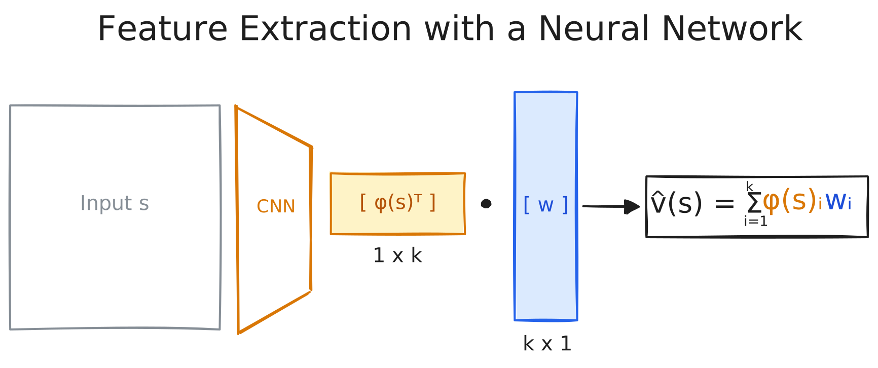
Setup

It’s instructive to decompose the value network into two parts: the last linear layer, with weights by $w$, and all prior layers, parametrized by $\theta$.

Figure 1: Decomposing the value network into representation layers $\theta$ and a linear layer $w$.

Features $\phi_\theta(s)$ are obtained by passing the state through the network, stopping at the last layer. The final value estimate is:

where $\hat{v}$ is parameterized by neural network weights $(\theta, w)$. The feature representation $\phi$ is a function, which takes any state (or more generally, any object in the state space) and returns a vector of length $k$.

Linear Value Function Learning

Before diving in to the full complexity of deep learning, let’s consider what we obtain when holding the features constant – that is, if we were to freeze $\phi$ and update $w$ only.

Let $\Phi$ be the matrix obtained by stacking the feature representations for all $N$ states. Thus, $\Phi$ is an $N \times k$ matrix where $k$ is the length of each feature vector. In general there are many more states than features, making $\Phi$ a “tall and skinny” matrix.

The space of all possible value functions we can represent is the column space of $\Phi$, also called $\text{span}(\Phi)$. In other words, all possible value estimates are of the form $\hat{v} = \Phi w$.

Best Linear Fit with the Projection Matrix

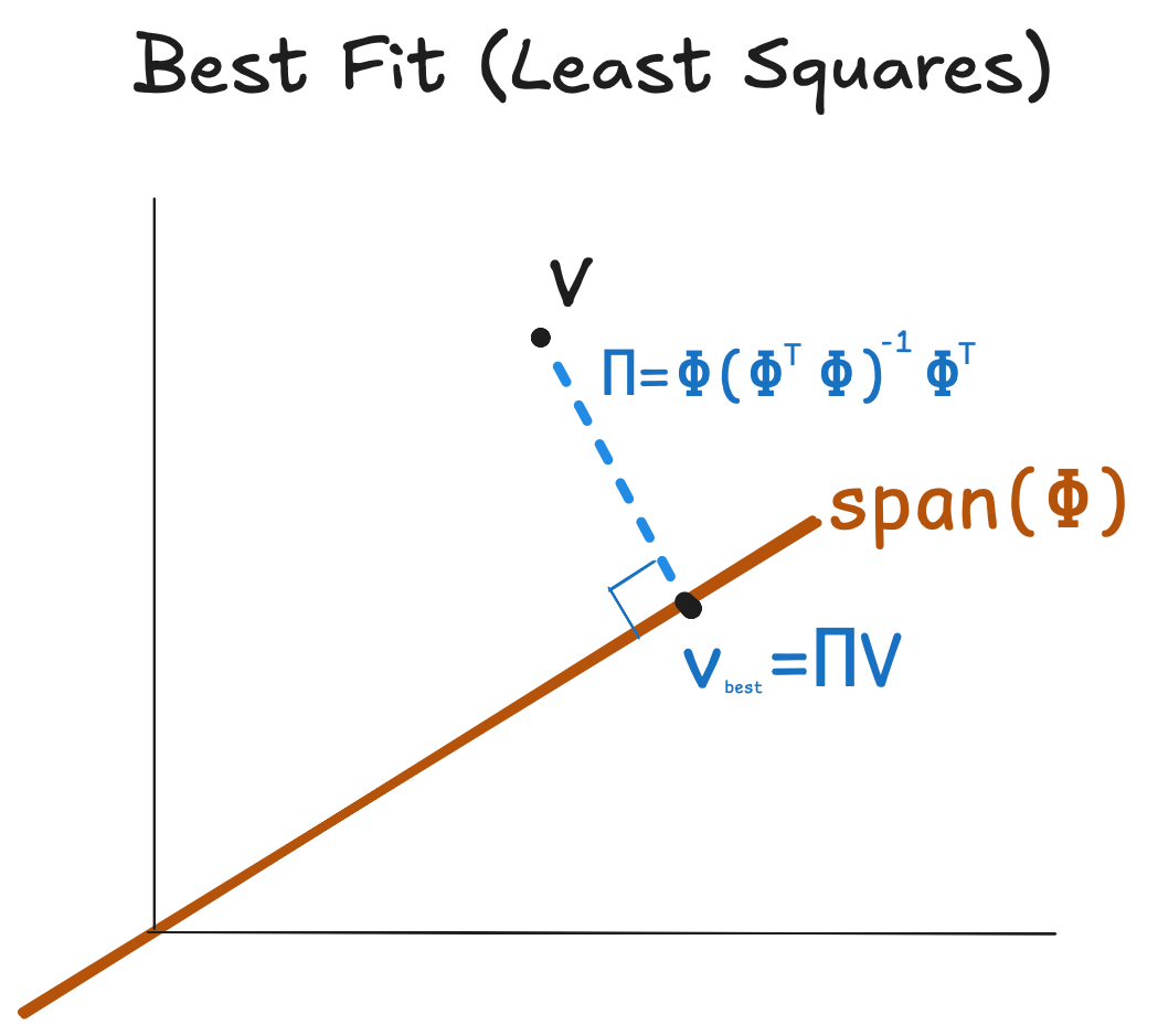
Suppose we had access to the true value function $V$ – a length $N$ vector where each element denotes a state value. Least squares theory tells us that the “best fit” that can be represented by $\Phi w$ for some $w$ would be given by:

where $\Pi = \Phi (\Phi^\top \Phi)^{-1} \Phi^\top$.

Figure 2: Geometric view of the best linear fit $\Pi V$ in the feature subspace $\text{span}(\Phi)$.

The above formulation treats all states equally. If we care about the value error differently across states, we can define a weighting distribution $\mu(s)$, and let $D = \text{diag}[\mu(s_1), \dots, \mu(s_N)]$ be a $N \times N$ square weighting matrix. This changes the projection matrix to:

\(\Pi = \Phi (\Phi^\top D \Phi)^{-1} \Phi^\top D\).

Note we still have $\hat{v}_{best} = \Pi V$.

The best linear fit provides a measure of the quality of our features. That is, the value error of $\hat{v}_{best}$ (the blue dotted line in the image) gets smaller exactly when our feature space $\text{span}(\Phi)$ gets closer to the true value function. Informally, $\text{Good Features} \iff \text{Best fit has low value error}$.

The value error vector $VE$, is defined as the difference between our fit and the true value function. For $v_{best}$ it is equal to the blue vector:

The length of this vector (weighting each state by $\mu$) gives us an overall estimate of the quality of our fit. The average value error – $\overline{VE}$ – is minimized by $v_{best}$.

This post focuses on TD learning, which refines a value estimate using its own current value. TD learning can be done by fitting targets based on a single transition, and is therefore much less noisy, generally leading to the strongest policy for most applications. However, it comes with complications. First, it introduces bias, because our target will generally not be the exact value function. Second, it doesn’t fit the ground truth, but instead a one-step refinement of its current guess.

The TD Learning Solution

TD Learning uses the Bellman operator, which, for any vector $v \in \mathbb{R}^N$, is $Tv = R + \gamma P v$. The Bellman operator is a contraction, and its fixed point is the true value function $V$. The fixed point equation is true only at the true value function $V$:

For other value functions $v$, we have a difference $Tv - V$. The contraction property implies that infinite application of $T$ will shrink this difference to zero:

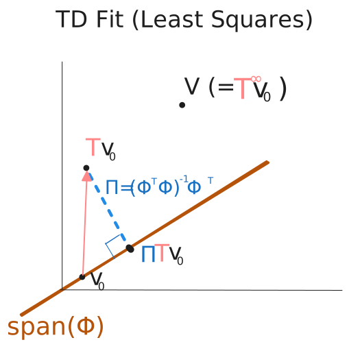
TD Learning attempts to fit the value function incrementally, starting with $v_0$ and repeatedly fitting $v_{i+1} \approx Tv_i$. In the linear case, this is done by approximating $T v_i$ with the best linear fit, yielding:

where $\Pi$ is the same projection matrix from before. The following picture shows this process of first applying the Bellman operator, followed by the projection matrix:

Figure 3: One step of linear TD: applying the Bellman Operator $T$, followed by the projection $\Pi$.

Under some assumptions¹, for fixed $\Phi$, repeated application of $\Pi T$ will, converge to a fixed point value estimate $v_{TD}$:

Note that $v_{TD} \neq v_{best}$ in general.

Deep TD Learning

Deep TD learning generalizes this procedure: repeatedly approximating $v_{i+1} \approx Tv_i$, with both $w$ and $\phi$ as free parameters. Both the target and representation evolve simultaneously.

Deep TD learning aims to reduce the length the following error, called the Bellman residual.

This is pink vector in the above images. The stop gradient, $sg(\cdot)$, is used since bootstrapping in this manner presents problem for gradient descent. In effect, TD learning drops the gradient $\nabla T v_i$, adjusting only $v_i$ – not $T v_i$. The update for any parameter $\omega \in (w, \theta)$ is:

Where $\alpha$ is a learning rate. Applying this rule, the expected change in weights and feature parameters at each round are:

Note that this treats $\theta$ as a column vector to keep the notation clean. At the linear fixed point $v_{TD}$, we have that $\Delta_w = 0$, since $\Phi$ is orthogonal to the TD error. However, $\Delta_\theta \neq 0$ in general, leading the features $\Phi$ to tilt towards the fixed $Tv_i$. This is how representation learning occurs for standard deep RL.

We consider an idealized version of TD learning, where the weights are always the least squares fit of the Bellman target: $\Phi w_i = \Pi_{\Phi_i} T v_i$. This allows us to focus on the update to the features, rather than the final linear layer.

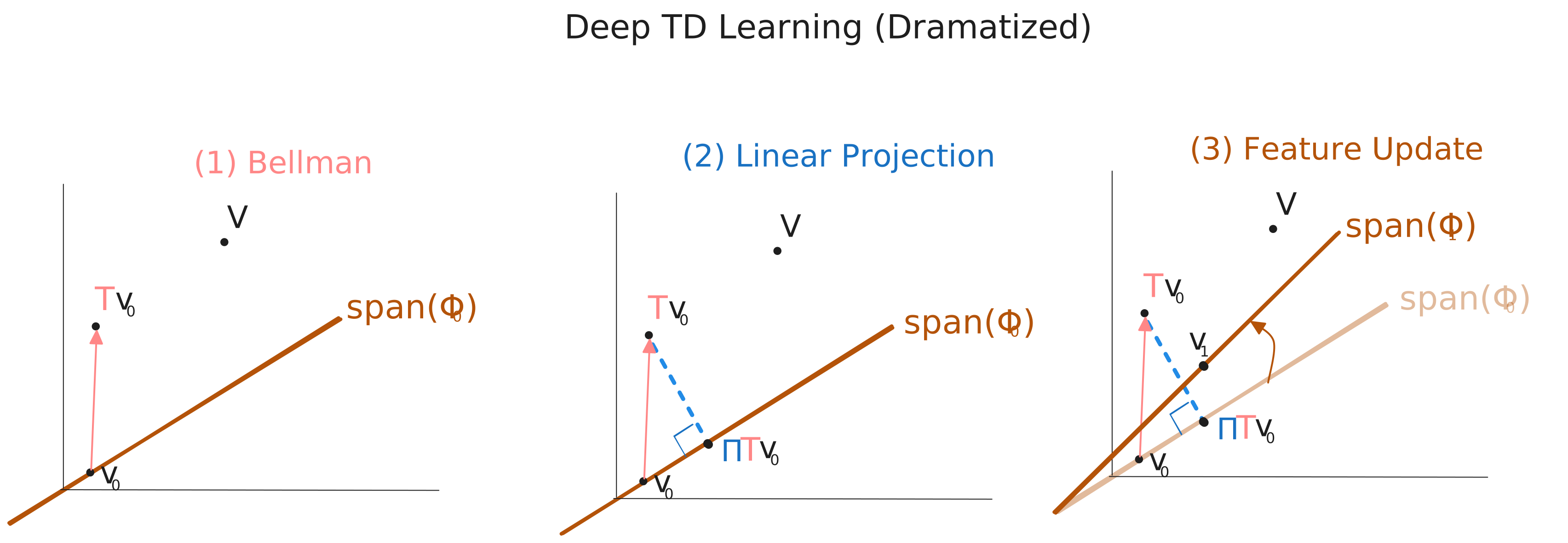
The following image breaks each update into three idealized steps. The first two steps are familiar from linear TD, but in the third step, the features change, adjusting $\Phi_1$ to $\Phi_2$ to shrink $Tv_i - \Pi T v_i$ .

Figure 4: One step of deep TD: features and weights both fit $Tv$

Does Deep TD Learning Improve the Representation?

Those dramatized images (that I made up) look pretty good! The final estimate $v_1$, which lives on the span of $\Phi_1$, is closer to both $T v_0$ and $V$! But looking at the image, we have no guarantee that $Tv_0$ and $V$ will be on the same side of the feature subspace. In that case, the update to $\Phi$ would actually be harmful for representing the true value function.

To more formally analyze this, let’s make some simplifying assumptions to help TD learning. First assume that $\mu$ corresponds to the on-policy distribution, which implies that $T$ is a contraction in the $\mu$-weighted norm². Given enough data and network capacity, it should be possible to achieve a perfect fit: $v_{i+1}= Tv_i$, in which case standard contraction arguments can be used to show that $\overline{VE}(v_i) \rightarrow 0$. This means that deep TD learning is fundamentally sound – at least asymptotically and under perfect conditions.

More interesting is what happens to the feature quality in each round, as measured by $\overline{VE}(v_{best})$. As we have already suggested, the feature quality can get worse, as stated in the following result:

Result: TD Learning does not always improve the representation: During update $i$ of Deep TD Learning, it’s possible that \(\|V - \Pi_{\Phi_i} V\|_\mu\) increases, even as \(\|Tv_i - \Pi_{\Phi_i} T v_i\|_\mu\) shrinks.

Geometrically, $\overline{VE}(v_{best})$ is made worse is when the true value function $V$ and $T v_i$ are on different sides of $\text{span}(\Phi)$. This is when the projection error on the Bellman target $\Pi Tv_i - Tv_i$ points in a different direction to the projection error for $v_{best}$. Algebraically, the condition:

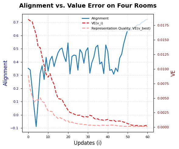
indicates that these two residuals point in different directions. This indicates that the update will improve feature quality if the the cosine similarity between these two vectors is higher, leading to the following alignment metric.

This might explain why regularization techniques that controlling the size of the gradient update are helpful empirically: by overfitting a single application of $T$ to a single value estimate, the features could be updated to make the overall value function worse compared to just doing linear TD from the beginning. Regularization like value target clipping and gradient norm clipping prevent the features from changing too much based on just a single application of the Bellman operator.

Under our assumptions, eventually the TD learning process will converge to the true value. At that point, we’ll have that $Tv_i - V = \gamma P (v_i - V)$ is small, since $v_i \approx V$. In short, the closer the value estimate gets to the true value, the less of a problem alignment will be. That said, in practice, a lack of alignment may prevent $v_i \rightarrow V$.

In summary, we have that, when applying TD learning under these idealized assumptions:

• The Current Predictor Improves: The value error $|V - v_i|_\mu$ always shrinks.
• The Representation Quality is not guaranteed to improve: The value error $|V-v_{best}|_\mu$ can grow if not aligned.

We can also ask whether the TD Fixed Point itself can get worse: is $|V - v_{TD}|$ guaranteed to improve? The worsening representation is certainly a plausible mechanism by which $v_{TD}$ could become worse.

Does $\overline{VE}(v_{best})$ even matter?

One might ask why we should care about this metric, if what we really care about is $\overline{VE}(v_i)$. The reason is that the final result of the optimization, assuming everything goes well, is the TD-fixed point. And, it is known that, as the representation improves, the TD-fixed point improves. It is known that if $V \in \text{span}(\Phi)$, the TD solution $v_{TD}$ will indeed be the true value function. Relatedly, a bound due to Scherrer 2010³ shows that when $\overline{VE}(v_{best})$ is small, $\overline{VE}(v_{TD})$ is controlled.

This motivates why $\overline{VE}(v_{best})$ is an important quantity, that standard deep TD learning may not optimize at each step.

Experiment

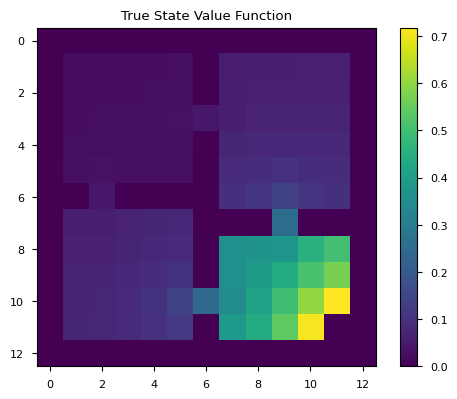
I perform online, batch TD learning to evaluate the random policy on Four Rooms. Four Rooms is a maze environment with $N =149$. I set the number of features $k=32$.

Figure 5: True Value Function for Four Rooms

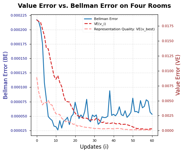
After each TD update, I compute the best solution $v_{best}$ for the current features and on-policy distribution, and compute the exact Bellman Error and Value Error. Recall the metrics:

• Bellman Error: $|Tv_i - v_i|_\mu^2$, indicates the degree that deep TD learning is shrinking the bellman residual.
• Value Error: $|V - v_i|_\mu^2$, indicates whether deep TD learning is improving its fit of the value function.
• Value Error of $v_{best}$: $|V - \Pi V |_\mu^2$, indicates whether the features are improving their proximity to $V$

Results

Asymptotically, the results are a success for TD learning. Given enough updates, we see that value error is brought extremely close to zero. This demonstrates that deep TD learning can indeed perform perfectly, even when introducing sampling and real-world deep learning dynamics.⁴

However, early in learning, there are some hiccups, where the representation quality actually gets worse. During this period (around $i=10$), the Bellman Error is being rapidly minimized, but the feature quality isn’t getting better.

Figure 6: VE and BE during learning

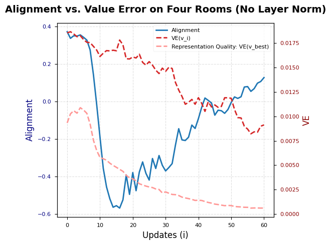
Interestingly, this bumpiness in $\overline{VE}(v_{best})$ happens when the alignment, as defined above, falls below zero, indicating that $Tv_i$ and $V$ are on opposite sides of the feature-space. However, for most of learning, they are on the same side!

Figure 6: VE alignment during learning

An ablation that that emphasizes caution

The above results are really promising! The network’s value error reached a minimum and the alignment generally stayed positive. However, things don’t look as nearly so good when one architectural change is made. The layer norm operation operates on each feature vector $\phi(s)\in \mathbb{R}^k$, subtracting the mean feature $\mu = \frac{1}{k}\sum_{j=1}^k \phi_j(s)$ and dividing by the feature standard deviation, $\sigma = \sqrt{ \frac{1}{k}\sum_{j=1}^k (\phi_j - \mu)^2}$. The experiments above take the output of a CNN in $\mathbb{R}^k$ and then apply a layer norm. We can hypothesize the layer norm helps prevent features from representing correlated concepts, or helps improves the variance of the features, helping the optimization of the weights due to conditioning.

Rather than focus on the layer norm, I just want to highlight how different the results become when this one architectural detail is changed. Without the layer norm, the alignment is poor, meaning that the update is often pointing away from the ground truth value. The representation quality is hurt (although its hard to tell at the scale of the graph, the minimum value of $VE(v_{best})$ is five times higher without the layer norm), and the final value estimate is 40 times worse than the same learning process with a layer norm.

Figure 7: VE alignment during learning with no layer norm.