Non-linear Value Learning
A key concept in RL is learning the value function with bootstrapping. But there are several objectives that all make use of bootstrapping, all of which differ in subtle but important ways. For instance, we have Bellman Error Minimization, TD Learning, Partially Fitted Value Iteration, not to mention Mean Squared Projected Bellman Error, oh my…
Making things more confusing, standard treatment of these algorithms (e.g. from Sutton and Barto) uses linear value function estimation. In that case, the span of the tangent line of the value estimate is the same as the hypothesis class itself. As we shall see, when the value estimate is not linear in its parameters, intuitions from linear RL break down.
In this post, I demonstrate the behavior of the following non-linear value function learning methods on the spiral MDP:
- Fitted Value Iteration (FVI)
- TD Learning
- Bellman Error Minimization
- Projected Bellman Error Minimization
- Monte Carlo / Supervised Value Learning
The Spiral MDP
Tsitsiklis and Van Roy devised a counterexample to demonstrate that TD learning fails on-policy with non-linear function approximation. As we will see, the spiral MDP also breaks fitted value iteration.
The problem is a Markov Reward Process (MRP) and value function estimator. The MRP has three states, thus the value function estimate, called \(v_\theta\), outputs a three-dimensional vector that depends on a single parameter \(\theta\). The reward is zero everywhere, meaning the true value is \(V^\pi = \mathbf{0}\). The magnitude of the estimate \(v_\theta\) approaches zero as \(\theta \rightarrow -\infty\).
The value function, and its estimate are in three dimensions. However, \(v_\theta\) will always live in a two-dimensional subspace. We visualize that subspace in Figure 1. The spiral shows our function class – all possible values of \(v_\theta\) (projected to the 2-D subspace). The sinusoidal curves show the value function as the \(\theta\) changes - with each color representing a different state value.
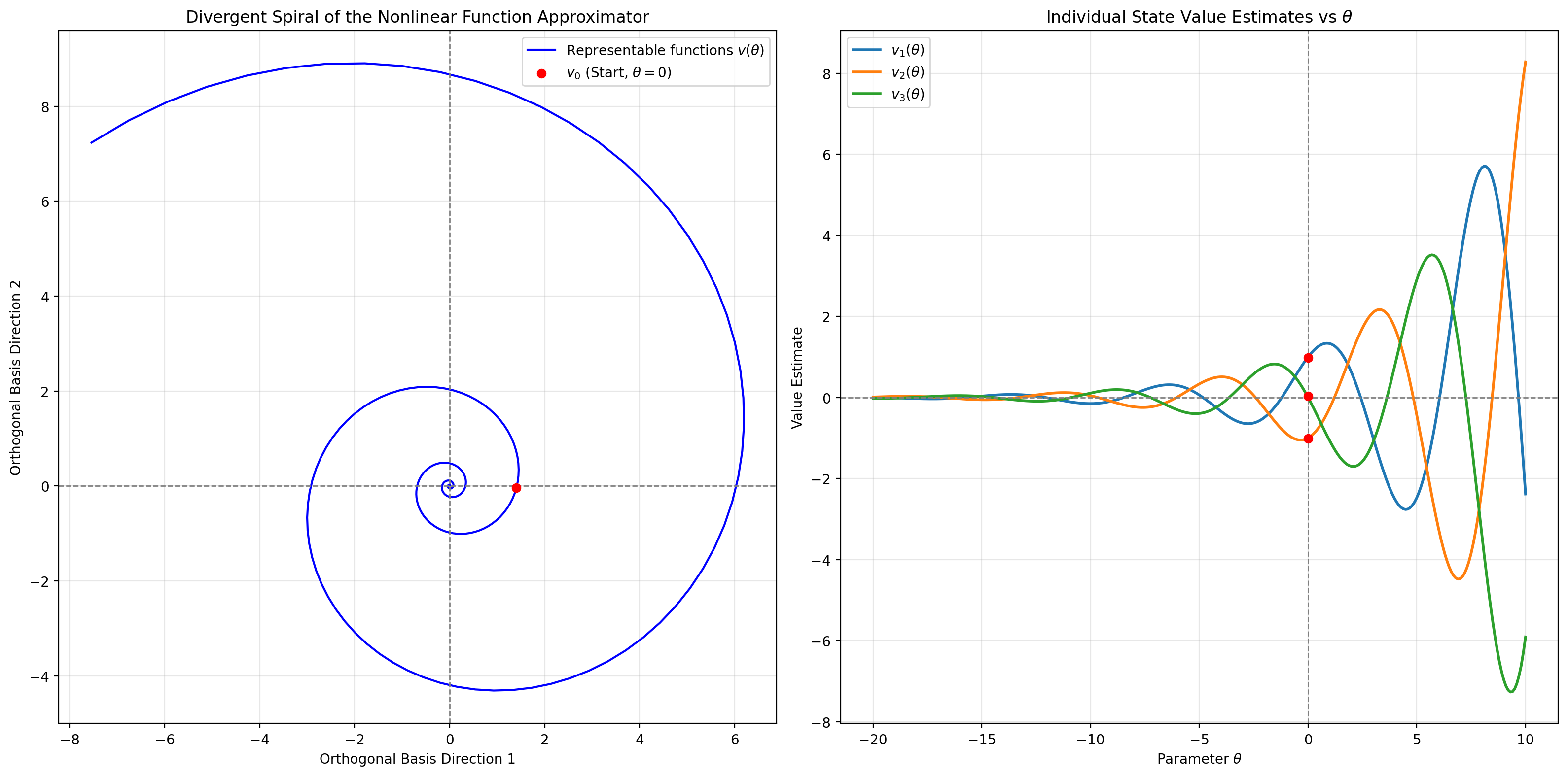
Figure 1: The Spiral MDP.
What’s nasty about this MRP – at least from the point of view of TD learning and friends – is that the Bellman Operator points towards the true value center, but when fitting it as a stationary target (like most bootstrapping methods), \(v_\theta\) fits the Bellman Estimate of the value, yet it diverges from \(V^\pi\).
A few technical details. First, the Bellman Operator is closed in this 2D space. For those who are curious why: \(\mathbf{1} =(1,1,1)^\intercal\) is a left eigenvector of \(P\) with eigenvalue 1. This implies that for any vector \(v\) orthogonal to \(\mathbf{1}\), \(Pv\) remains orthogonal to \(\mathbf{1}\), since \(\mathbf{1}^\intercal P v = \mathbf{1}^\intercal v = 0\).
Technical detail 2: The state-visitation distribution in the spiral MDP is exactly one third times the identity. Thus the on-policy weighted distance reduces to a constant scalar times the Euclidean distance. Technically, all inner products should be weighted by the on-policy distribution (stored in the matrix \(D\) in my earlier posts), but because \(D = \frac{1}{3}I\), I ignore it in this post. See the final section of the original paper for the description of the MRP.
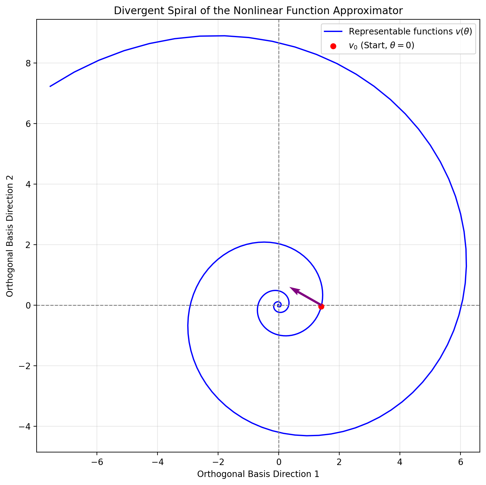
Figure 2: Bellman Operator.
Algorithm 1: (Partially) Fitted Value Iteration (FVI)
(Partially) Fitted Value Iteration (FVI) is the most common value learning algorithm in deep RL. For example, DQN and PPO both perform FVI. Generally, FVI is thought of as a batch algorithm. It repeatedly fits the Bellman Operator. In expectation, it works as follows:
Algorithm: FVI
Repeat:
0. Initialize Target Network u <- v.
1. Estimate Tu = R + γPu.
2. Compute v by minimizing the length of Tu-v.
The distinction between batch FVI and PFVI lies entirely in the final step, when a new value estimate is obtained as \(v_\theta \gets \operatorname{argmin}_{v_\theta} \|Tu - v_\theta\|^2\). In classic linear FVI, the best fit for \(\theta\) can be obtained using least squares regression.
Deep variants perform gradient descent on \(\theta\). But for how many gradient updates? If we fit \(\theta\) for just one step of gradient descent, we get TD learning. If we run gradient descent until convergence, we get full batch FVI. The crux of the problem is that gradient descent doesn’t give us a global minimum. And the local optimum obtained is unfortunately worse than what we started with.
I run FVI on the spiral problem, with 200 gradient steps per Bellman update. The learning dynamics shown are in Figure 3. The left panel shows the parameter value with each update – notice that it is diverging away from the best estimate \(\theta^* = -\infty\). The middle panel shows the trajectory on the spiral. The trajectory appears to be going in the wrong direction, despite a better fit being available in the function class. How can this be? As the right panel shows: the loss landscape is non-convex. The global minimum estimator appears to be far to the right, around \(\theta=-5\). But there is a different local minimum in the other direction. Because the loss landscape is non-convex, each round of FVI gets further away from \(Tv\).
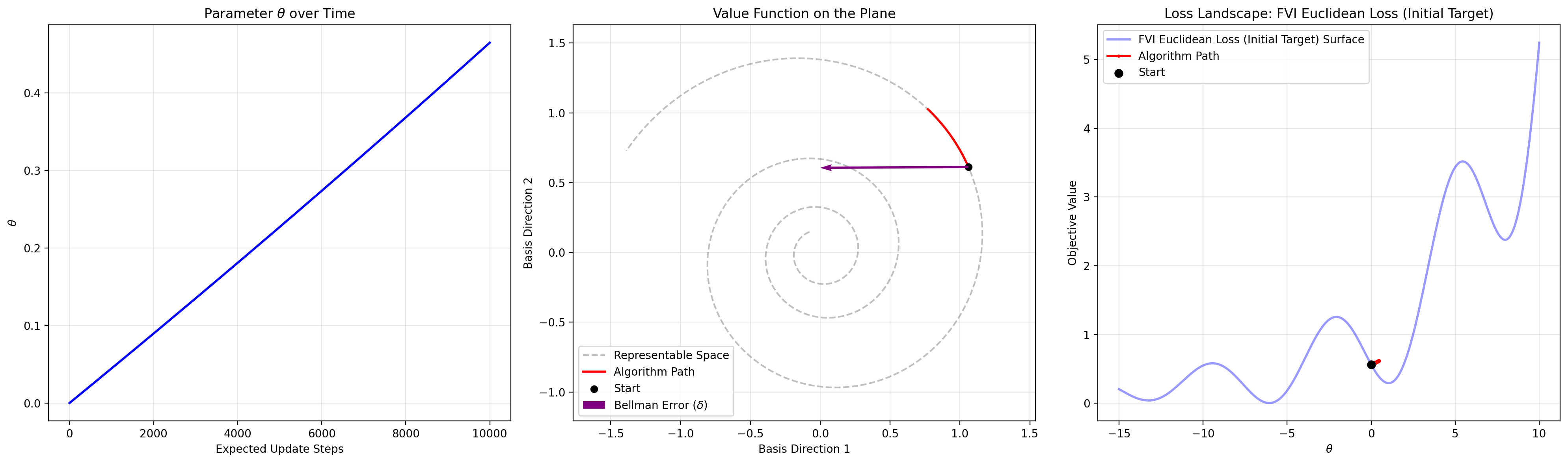
Figure 3: Learning Dynamics of FVI.
Because our \(v_\theta\) is non-convex, fitting the Bellman operator can lead to a worse value estimate, breaking the contraction argument for why standard exact value iteration converges. In short, the “fitted” component of FVI breaks the guarantee of value iteration. Figure 4 shows a longer run. Note that the parameters traverse the fixed loss landscape, since the loss changes with each application of \(T\) (but I only show the first loss).
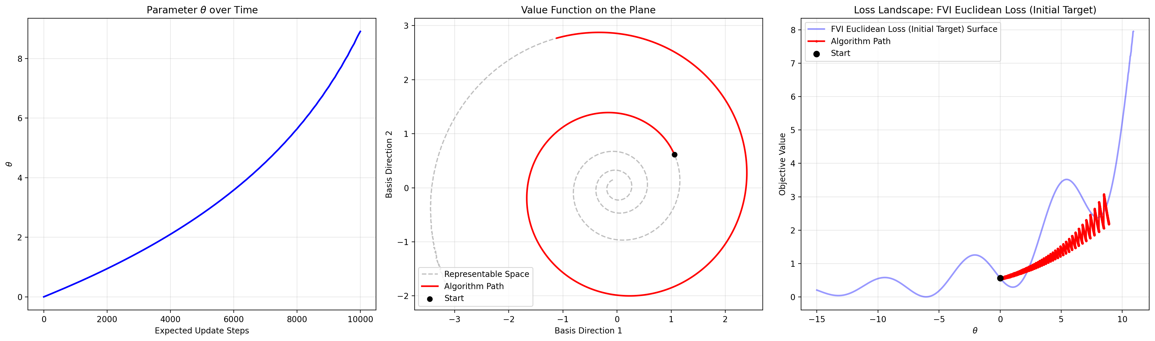
Figure 4: Longer Run of FVI.
Algorithm 2: TD Learning
Tsitsiklis and Van Roy’s original 1997 paper analyzed TD learning. As mentioned above, TD learning takes a single gradient step to fit the Bellman Operator before updating the value function. A single gradient step is a locally linear approximation to the true optimal direction. As such, each step of TD learning can be understood as taking a small step towards the projection of \(Tv_\theta\) onto the space orthogonal to the tangent line of \(v_\theta\).
Figure 5 shows the dynamics of TD learning. Again, a single application of the Bellman Operator to the starting value estimate is shown in purple. The green line shows the projection of \(Tv_\theta\) onto the span of \(\nabla_\theta v\) (a length 3 vector with entries \(\frac{dv}{d\theta}(s_i)\) for each state). Notice that this line points away from the center due to the direction of the spiral and angle of \(T\).
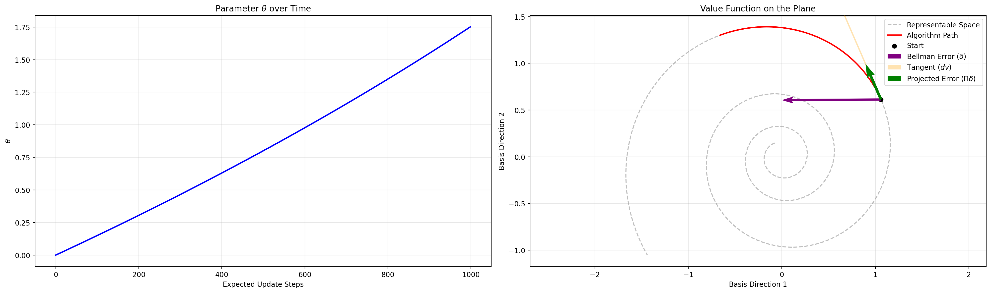
Figure 5: TD Learning.
def td_update(θ, v, dv, α):
    δ = T(v) - v
    θ = θ + α * dv.T @ δ
    return θ
Note that in the linear case, the span of the tangent line is the space of representable functions. In this case, FVI and TD learning have the same fixed point.
Algorithm 3: Bellman Error Minimization (BEM)
Bellman Error Minimization (Baird, L. (1995)) solves \(\min_{\theta} \|Tv_\theta - v_\theta\|_2^2\). This looks a lot like TD learning and FVI. The key difference is that BEM differentiates both \(v_\theta\) AND \(T v_\theta\) with respect to \(\theta\). Whereas TD learning and FVI fix \(T v_\theta\) (e.g. with a target network).
\[\begin{align} \nabla_\theta \|Tv_\theta - v_\theta\|_2^2 &= 2(Tv_\theta - v_\theta)^\intercal \nabla_\theta (Tv_\theta - v_\theta) \\ &= 2 \delta^\intercal (\nabla_\theta T v_\theta - \nabla_\theta v_\theta) \end{align}\]The presence of \(\nabla_\theta T v_\theta\) means that BEM techniques must incorporate information about how \(Tv\) changes with \(v\). More precisely, BEM methods must estimate \(P \nabla_\theta v_\theta\) – the expected value of the gradient one step into the future – as well as \(\delta\), and take their product. Since the expectation of a product does not equal the product of expectations, a naive sample-based update requires two independent transitions from the same state (the double sampling issue). However, just as in GTD methods, one can circumvent double sampling by introducing an auxiliary weight vector to estimate the expected future gradient product without requiring two next-state samples. In our experiments on the spiral problem, we can compute all terms in the gradient exactly.
Results are shown in Figure 6. Note that BEM succeeds on this problem.
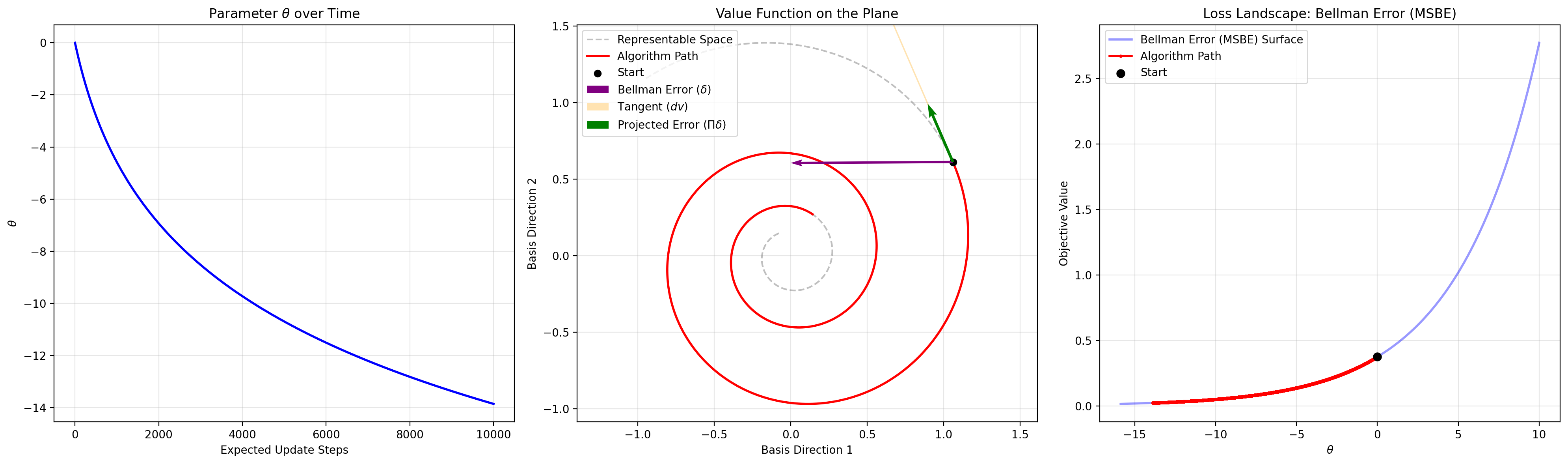
Figure 6: Bellman Error Minimization.
Algorithm 4: Mean Squared Projected Bellman Error (MSPBE)
The MSPBE is the length of the green vector in Figure 5. Letting \(\Pi_\theta\) be the linear projection onto the span of \(\nabla_\theta v\), we have:
\[\text{MSPBE} = \| \Pi_\theta (T v_\theta - v_\theta) \|^2 = \| \Pi_\theta \delta_\theta \|^2 = \delta_\theta^\intercal \Pi_\theta \delta_\theta\]Since we have just one parameter, \(\Pi_\theta\) is the \(3\times3\) matrix:
\[\Pi_\theta = \frac{1}{\|\nabla_\theta v\|^2} (\nabla_\theta v) (\nabla_\theta v)^\intercal\]Plugging this in, we the squared TD learning update, divided by the squared length of the tangent vector \(\|\nabla_\theta v\|^2\):
\[\begin{align} \text{MSPBE} &= \frac{1}{\|\nabla_\theta v\|^2} (\delta_\theta^\intercal \nabla_\theta v)^2. \end{align}\]There are numerous issues minimizing this quantity. For one, the gradient of the MSPBE contains the product of value network Hessians. Secondly, it once again requires estimating \(P \nabla_\theta v_\theta\) – in other words, it must know how $v_\theta$ changes as a local function of \(\theta\). This also requires addressing the double sampling issue. Methods that minimize the MSPBE avoid double sampling by training an estimator to predict the Bellman error.
For our toy problem, we can compute the gradient of the MSPBE exactly - and find that it works! At each step, it can be thought of as changing \(\theta\), re-applying the Bellman operator, and measuring the length of the green line. The right panel shows the true MSPBE - or the length of the green vector - as learning progresses.
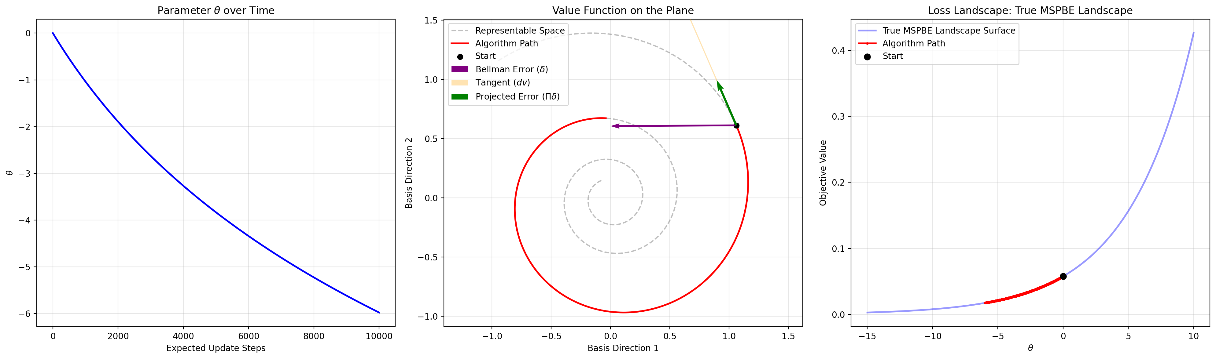
Figure 7: MSPBE Minimization.
Algorithm 5: Monte Carlo
Removing all sampling noise, Monte Carlo value learning is just supervised learning of the center of the circle. Does this suffer from a highly non-convex landscape like FVI?
It does not. As \(\theta\) decreases, the error monotonically decreases as well, leading to a convex loss landscape. Note that its loss, shown in the fourth panel of Figure 8, has quite a similar shape to the MSPBE error, which is shown in the third panel.
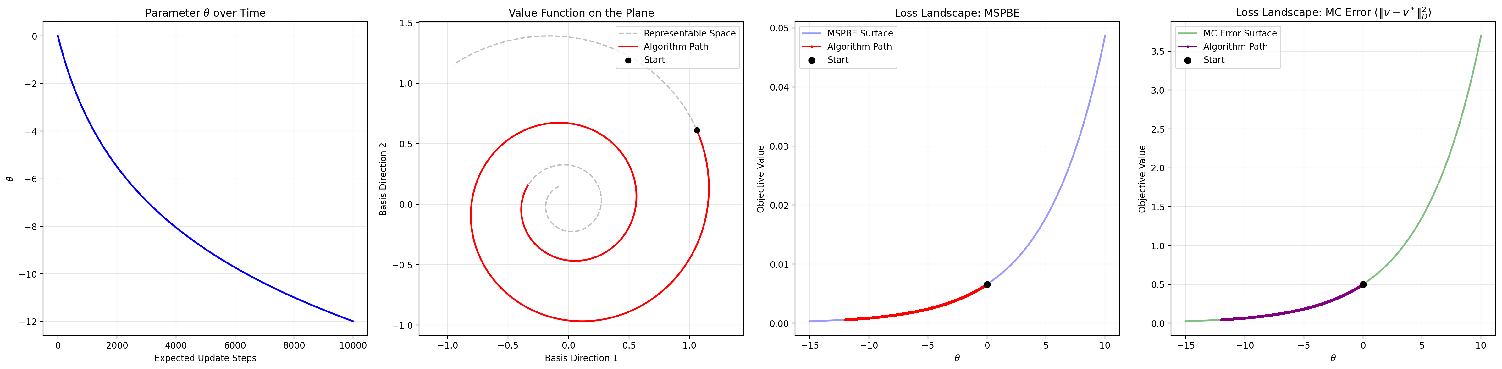
Figure 8: Monte Carlo / Value Error Minimization.
Summary
In short, all one-step methods either fail (TD and FVI), or face the double sampling issue (BEM and MSPBE minimization). In our experiments, we take advantage of access to the true transition matrix and reward function to bypass the double sampling issue. Additionally, we get strong performance from multi-step methods like MC / VEM, due to the absence of sampling variance.