This post investigates Deep Temporal Difference (TD) learning as used to fit the value function in RL. It first provides a geometric explanation of deep TD learning. This highlights that deep TD learning does not directly optimize its representation to predict the true value function. Instead, it predicts a moving Bellman target. Whether this indirectly improves representation depends on how aligned those two objectives are.

The main question of this post is:

Does TD learning improve the representation’s ability to represent the true value function?

I make a set of idealized assumptions, under which the value predictions due to deep TD learning are guaranteed to improve. I show, however, that adjusting the features to fit the Bellman target does not necessarily improve the representation. A simple geometric argument shows that the quality of the final representation depends on the alignment between the TD target and the true value function.

I show with a simple experiment on four rooms that the alignment isn’t always an issue, and TD learning can still succeed! But, another experiment has poor alignment and signfiicantly worse value learning.

Along the way, I frame the process of deep TD learning geometrically, visualizing the state space, where the true value lives, and the smaller subspace to which the estimate is confined. We’ll end with a closer look at a real example. So let’s go!

Setup

It’s instructive to decompose the value network into two parts: the last linear layer, with weights by $w$, and all prior layers, parametrized by $\theta$.

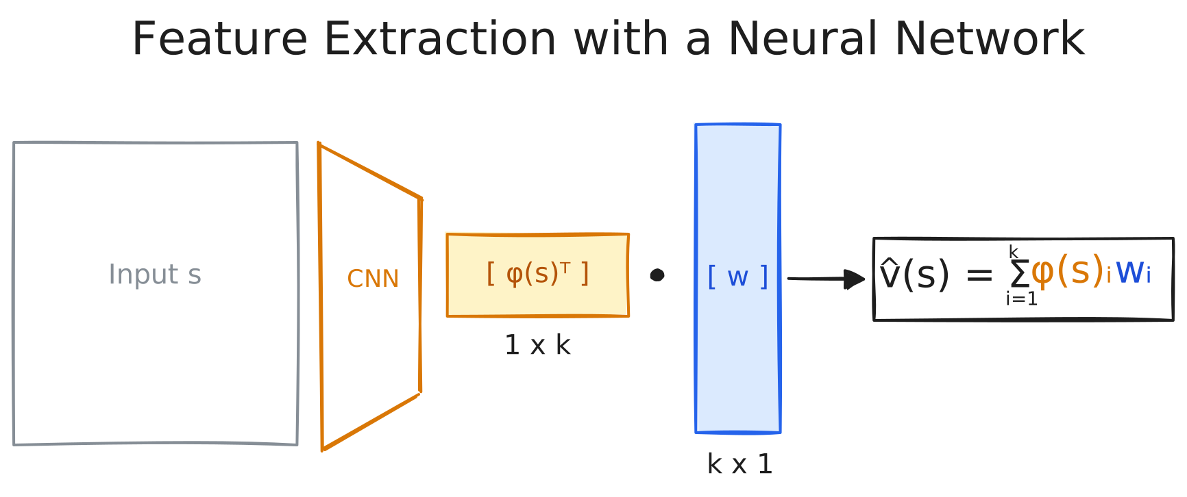
Figure 1: Decomposing the value network into representation layers $\theta$ and a linear layer $w$.

Features $\phi_\theta(s)$ are obtained by passing the state through the network, stopping at the last layer. The final value estimate is:

\[\begin{aligned} \hat{v}(s) = \phi(s)^\top w \end{aligned}\]

where $\hat{v}$ is parameterized by neural network weights $(\theta, w)$. The feature representation $\phi$ is a function, which takes any state (or more generally, any object in the state space) and returns a vector of length $k$.

Linear Value Function Learning

Before diving in to the full complexity of deep learning, let’s consider what we obtain when holding the features constant – that is, if we were to freeze $\phi$ and update $w$ only.

Let $\Phi$ be the matrix obtained by stacking the feature representations for all $N$ states. Thus, $\Phi$ is an $N \times k$ matrix where $k$ is the length of each feature vector. In general there are many more states than features, making $\Phi$ a “tall and skinny” matrix.

The space of all possible value functions we can represent is the column space of $\Phi$, also called $\text{span}(\Phi)$. In other words, all possible value estimates are of the form $\hat{v} = \Phi w$.

\[\Phi = \begin{bmatrix} \longleftarrow & \phi(s_1)^T & \longrightarrow \\ \longleftarrow & \phi(s_2)^T & \longrightarrow \\ & \vdots & \\ \longleftarrow & \phi(s_N)^T & \longrightarrow \end{bmatrix}\]

Best Linear Fit with the Projection Matrix

Suppose we had access to the true value function $V$ – a length $N$ vector where each element denotes a state value. Least squares theory tells us that the “best fit” that can be represented by $\Phi w$ for some $w$ would be given by:

\[\hat{v}_{best} = \Pi V\]

where $\Pi = \Phi (\Phi^\top \Phi)^{-1} \Phi^\top$.

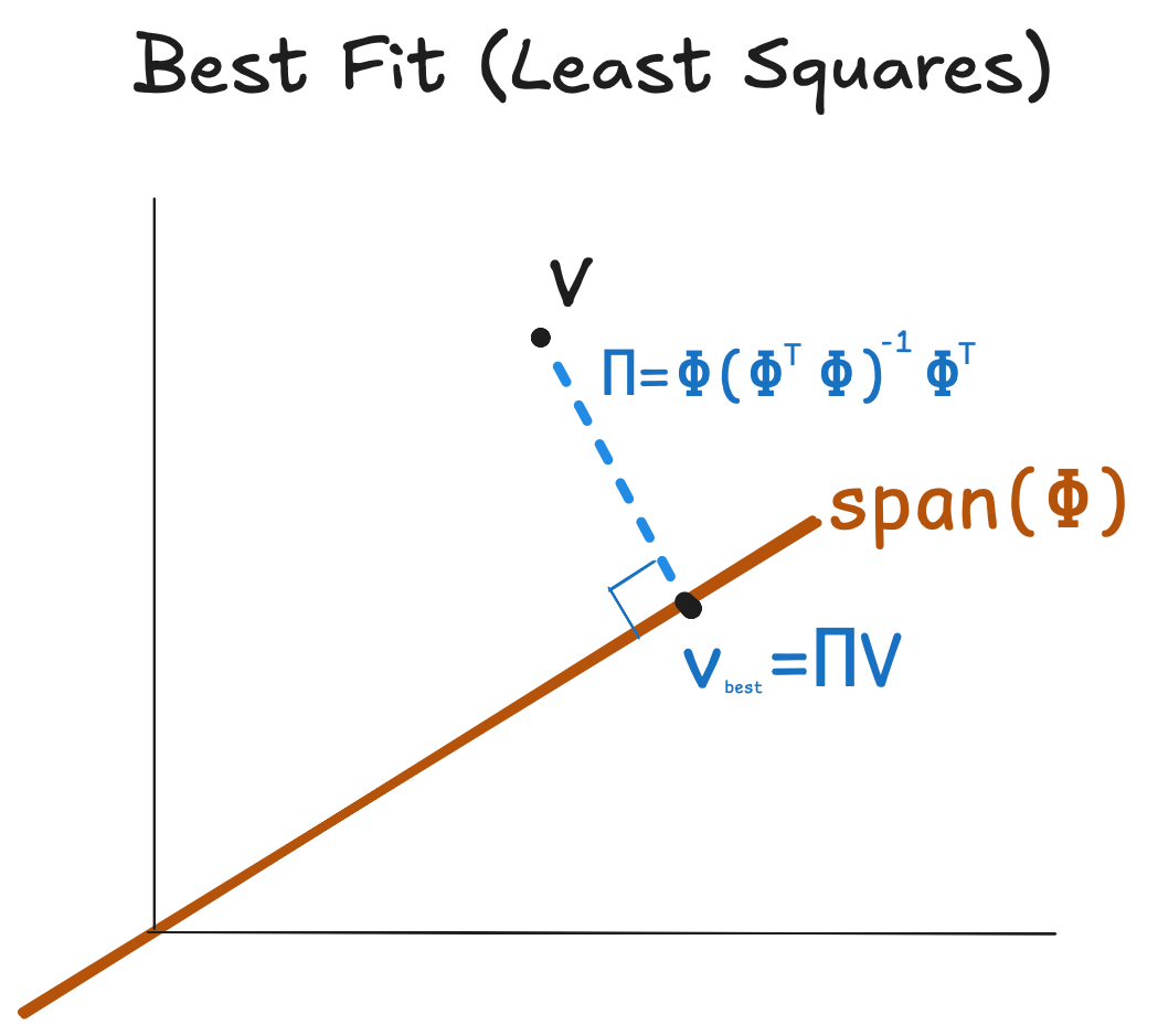
Figure 2: Geometric view of the best linear fit $\Pi V$ in the feature subspace $\text{span}(\Phi)$.

The above formulation treats all states equally. If we care about the value error differently across states, we can define a weighting distribution $\mu(s)$, and let $D = \text{diag}[\mu(s_1), \dots, \mu(s_N)]$ be a $N \times N$ square weighting matrix. This changes the projection matrix to:

$\Pi = \Phi (\Phi^\top D \Phi)^{-1} \Phi^\top D$.

Note we still have $\hat{v}_{best} = \Pi V$.

The best linear fit provides a measure of the quality of our features. That is, the value error of $\hat{v}_{best}$ (the blue dotted line in the image) gets smaller exactly when our feature space $\text{span}(\Phi)$ gets closer to the true value function. Informally, $\text{Good Features} \iff \text{Best fit has low value error}$.

The value error vector $VE$, is defined as the difference between our fit and the true value function. For $v_{best}$ it is equal to the blue vector:

\[VE(v_{best}) = V - \Pi V\]

The length of this vector (weighting each state by $\mu$) gives us an overall estimate of the quality of our fit. The average value error – $\overline{VE}$ – is minimized by $v_{best}$.

\[\overline{VE}(v) = \sum_s \mu(s) (V(s) - v(s))^2 = \|V - v\|_\mu^2\]

This post focuses on TD learning, which refines a value estimate using its own current value. TD learning can be done by fitting targets based on a single transition, and is therefore much less noisy, generally leading to the strongest policy for most applications. However, it comes with complications. First, it introduces bias, because our target will generally not be the exact value function. Second, it doesn’t fit the ground truth, but instead a one-step refinement of its current guess.

The TD Learning Solution

TD Learning uses the Bellman operator, which, for any vector $v \in \mathbb{R}^N$, is $Tv = R + \gamma P v$. The Bellman operator is a contraction, and its fixed point is the true value function $V$. The fixed point equation is true only at the true value function $V$:

\[TV = V \quad (\text{system of N equations})\]

For other value functions $v$, we have a difference $Tv - V$. The contraction property implies that infinite application of $T$ will shrink this difference to zero:

\[T^\infty v = V\]

TD Learning attempts to fit the value function incrementally, starting with $v_0$ and repeatedly fitting $v_{i+1} \approx Tv_i$. In the linear case, this is done by approximating $T v_i$ with the best linear fit, yielding:

\[v_{i+1} = \Pi T v_i\]

where $\Pi$ is the same projection matrix from before. The following picture shows this process of first applying the Bellman operator, followed by the projection matrix:

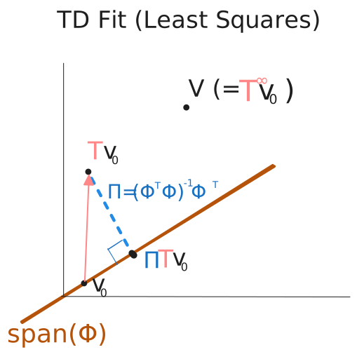
Figure 3: One step of linear TD: applying the Bellman Operator $T$, followed by the projection $\Pi$.

Under some assumptions¹, for fixed $\Phi$, repeated application of $\Pi T$ will, converge to a fixed point value estimate $v_{TD}$:

\[v_{TD} = \Pi T v_{TD}\]

Note that $v_{TD} \neq v_{best}$ in general.

Deep TD Learning

Deep TD learning generalizes this procedure: repeatedly approximating $v_{i+1} \approx Tv_i$, with both $w$ and $\phi$ as free parameters. Both the target and representation evolve simultaneously.

Deep TD learning aims to reduce the length the following error, called the Bellman residual.

\[(\text{sg}(Tv_{i}) - v_i)\]

This is pink vector in the above images. The stop gradient, $sg(\cdot)$, is used since bootstrapping in this manner presents problem for gradient descent. In effect, TD learning drops the gradient $\nabla T v_i$, adjusting only $v_i$ – not $T v_i$. The update for any parameter $\omega \in (w, \theta)$ is:

\[\omega_{i+1} = \omega_i + \alpha (Tv_{i} - v_i) \cdot \nabla_\omega v_i\]

Where $\alpha$ is a learning rate. Applying this rule, the expected change in weights and feature parameters at each round are:

\[\begin{aligned} \Delta_ w &\propto \Phi^\top D (Tv_{i} - v_i) \\ \Delta_\theta &\propto (\nabla_\theta \Phi w)^\top D (Tv_{i} - v_i)\ \end{aligned}\]

Note that this treats $\theta$ as a column vector to keep the notation clean. At the linear fixed point $v_{TD}$, we have that $\Delta_w = 0$, since $\Phi$ is orthogonal to the TD error. However, $\Delta_\theta \neq 0$ in general, leading the features $\Phi$ to tilt towards the fixed $Tv_i$. This is how representation learning occurs for standard deep RL.

We consider an idealized version of TD learning, where the weights are always the least squares fit of the Bellman target: $\Phi w_i = \Pi_{\Phi_i} T v_i$. This allows us to focus on the update to the features, rather than the final linear layer.

The following image breaks each update into three idealized steps. The first two steps are familiar from linear TD, but in the third step, the features change, adjusting $\Phi_1$ to $\Phi_2$ to shrink $Tv_i - \Pi T v_i$ .

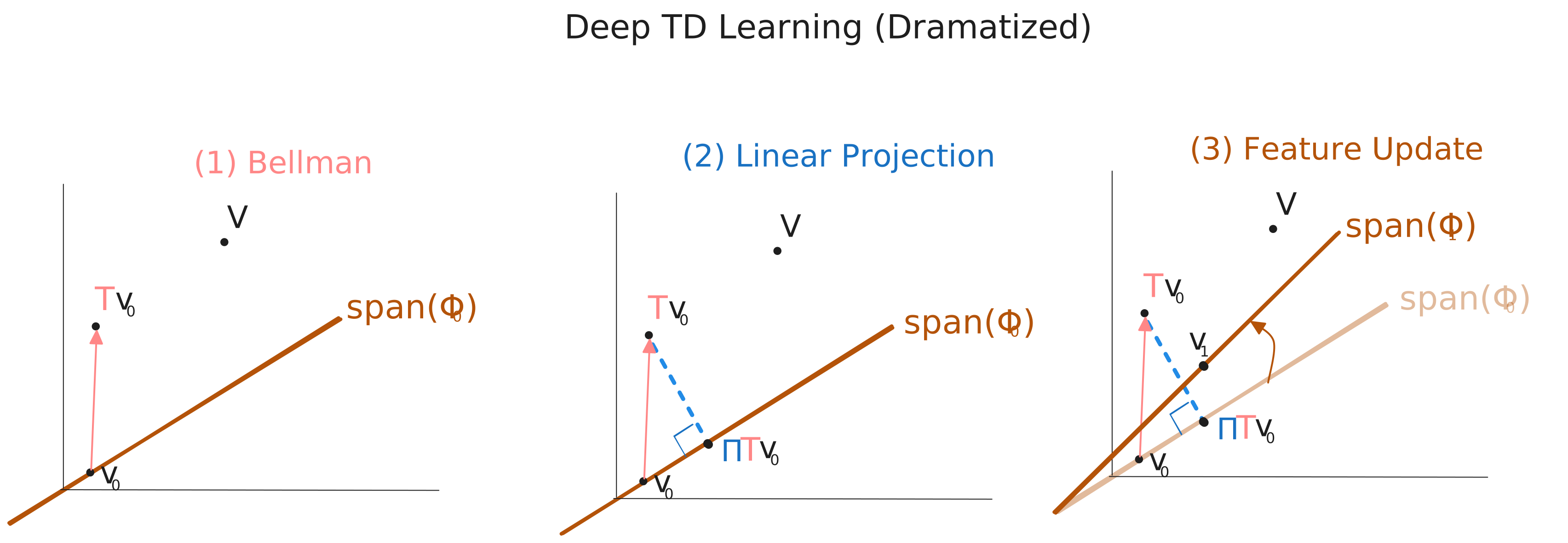
Figure 4: One step of deep TD: features and weights both fit $Tv$

Does Deep TD Learning Improve the Representation?

Those dramatized images (that I made up) look pretty good! The final estimate $v_1$, which lives on the span of $\Phi_1$, is closer to both $T v_0$ and $V$! But looking at the image, we have no guarantee that $Tv_0$ and $V$ will be on the same side of the feature subspace. In that case, the update to $\Phi$ would actually be harmful for representing the true value function.

To more formally analyze this, let’s make some simplifying assumptions to help TD learning. First assume that $\mu$ corresponds to the on-policy distribution, which implies that $T$ is a contraction in the $\mu$-weighted norm². Given enough data and network capacity, it should be possible to achieve a perfect fit: $v_{i+1}= Tv_i$, in which case standard contraction arguments can be used to show that $\overline{VE}(v_i) \rightarrow 0$. This means that deep TD learning is fundamentally sound – at least asymptotically and under perfect conditions.

More interesting is what happens to the feature quality in each round, as measured by $\overline{VE}(v_{best})$. As we have already suggested, the feature quality can get worse, as stated in the following result:

Result: TD Learning does not always improve the representation: During update $i$ of Deep TD Learning, it’s possible that $\|V - \Pi_{\Phi_i} V\|_\mu$ increases, even as $\|Tv_i - \Pi_{\Phi_i} T v_i\|_\mu$ shrinks.

Geometrically, $\overline{VE}(v_{best})$ is made worse is when the true value function $V$ and $T v_i$ are on different sides of $\text{span}(\Phi)$. This is when the projection error on the Bellman target $\Pi Tv_i - Tv_i$ points in a different direction to the projection error for $v_{best}$. Algebraically, the condition:

\[(\Pi V-V)^\top D (\Pi T v_i - Tv_i) < 0\]

indicates that these two residuals point in different directions. This indicates that the update will improve feature quality if the the cosine similarity between these two vectors is higher, leading to the following alignment metric.

\[\text{alignment} = \frac{(\Pi V-V)^\top D (\Pi T v_i - Tv_i)}{\| \Pi V-V\|_D \|\Pi Tv_i-Tv_i \|_D}\]

This might explain why regularization techniques that controlling the size of the gradient update are helpful empirically: by overfitting a single application of $T$ to a single value estimate, the features could be updated to make the overall value function worse compared to just doing linear TD from the beginning. Regularization like value target clipping and gradient norm clipping prevent the features from changing too much based on just a single application of the Bellman operator.

Under our assumptions, eventually the TD learning process will converge to the true value. At that point, we’ll have that $Tv_i - V = \gamma P (v_i - V)$ is small, since $v_i \approx V$. In short, the closer the value estimate gets to the true value, the less of a problem alignment will be. That said, in practice, a lack of alignment may prevent $v_i \rightarrow V$.

In summary, we have that, when applying TD learning under these idealized assumptions:

The Current Predictor Improves: The value error $|V - v_i|_\mu$ always shrinks.
The Representation Quality is not guaranteed to improve: The value error $|V-v_{best}|_\mu$ can grow if not aligned.

We can also ask whether the TD Fixed Point itself can get worse: is $|V - v_{TD}|$ guaranteed to improve? The worsening representation is certainly a plausible mechanism by which $v_{TD}$ could become worse.

Does $\overline{VE}(v_{best})$ even matter?

One might ask why we should care about this metric, if what we really care about is $\overline{VE}(v_i)$. The reason is that the final result of the optimization, assuming everything goes well, is the TD-fixed point. And, it is known that, as the representation improves, the TD-fixed point improves. It is known that if $V \in \text{span}(\Phi)$, the TD solution $v_{TD}$ will indeed be the true value function. Relatedly, a bound due to Scherrer 2010³ shows that when $\overline{VE}(v_{best})$ is small, $\overline{VE}(v_{TD})$ is controlled.

This motivates why $\overline{VE}(v_{best})$ is an important quantity, that standard deep TD learning may not optimize at each step.

Experiment

I perform online, batch TD learning to evaluate the random policy on Four Rooms. Four Rooms is a maze environment with $N =149$. I set the number of features $k=32$.

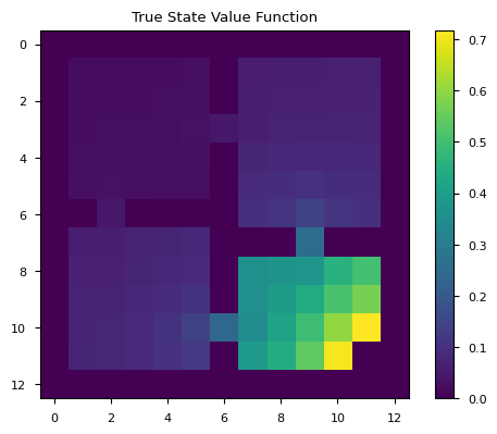
Figure 5: True Value Function for Four Rooms

After each TD update, I compute the best solution $v_{best}$ for the current features and on-policy distribution, and compute the exact Bellman Error and Value Error. Recall the metrics:

Bellman Error: $|Tv_i - v_i|_\mu^2$, indicates the degree that deep TD learning is shrinking the bellman residual.
Value Error: $|V - v_i|_\mu^2$, indicates whether deep TD learning is improving its fit of the value function.
Value Error of $v_{best}$: $|V - \Pi V |_\mu^2$, indicates whether the features are improving their proximity to $V$

Results

Asymptotically, the results are a success for TD learning. Given enough updates, we see that value error is brought extremely close to zero. This demonstrates that deep TD learning can indeed perform perfectly, even when introducing sampling and real-world deep learning dynamics.⁴

However, early in learning, there are some hiccups, where the representation quality actually gets worse. During this period (around $i=10$), the Bellman Error is being rapidly minimized, but the feature quality isn’t getting better.

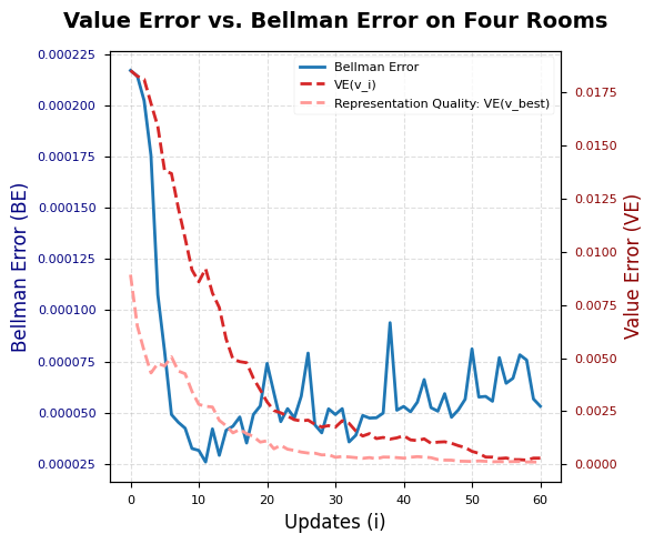
Figure 6: VE and BE during learning

Interestingly, this bumpiness in $\overline{VE}(v_{best})$ happens when the alignment, as defined above, falls below zero, indicating that $Tv_i$ and $V$ are on opposite sides of the feature-space. However, for most of learning, they are on the same side!

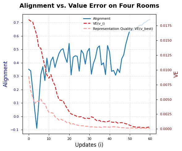
Figure 6: VE alignment during learning

An ablation that that emphasizes caution

The above results are really promising! The network’s value error reached a minimum and the alignment generally stayed positive. However, things don’t look as nearly so good when one architectural change is made. The layer norm operation operates on each feature vector $\phi(s)\in \mathbb{R}^k$, subtracting the mean feature $\mu = \frac{1}{k}\sum_{j=1}^k \phi_j(s)$ and dividing by the feature standard deviation, $\sigma = \sqrt{ \frac{1}{k}\sum_{j=1}^k (\phi_j - \mu)^2}$. The experiments above take the output of a CNN in $\mathbb{R}^k$ and then apply a layer norm. We can hypothesize the layer norm helps prevent features from representing correlated concepts, or helps improves the variance of the features, helping the optimization of the weights due to conditioning.

Rather than focus on the layer norm, I just want to highlight how different the results become when this one architectural detail is changed. Without the layer norm, the alignment is poor, meaning that the update is often pointing away from the ground truth value. The representation quality is hurt (although its hard to tell at the scale of the graph, the minimum value of $VE(v_{best})$ is five times higher without the layer norm), and the final value estimate is 40 times worse than the same learning process with a layer norm.

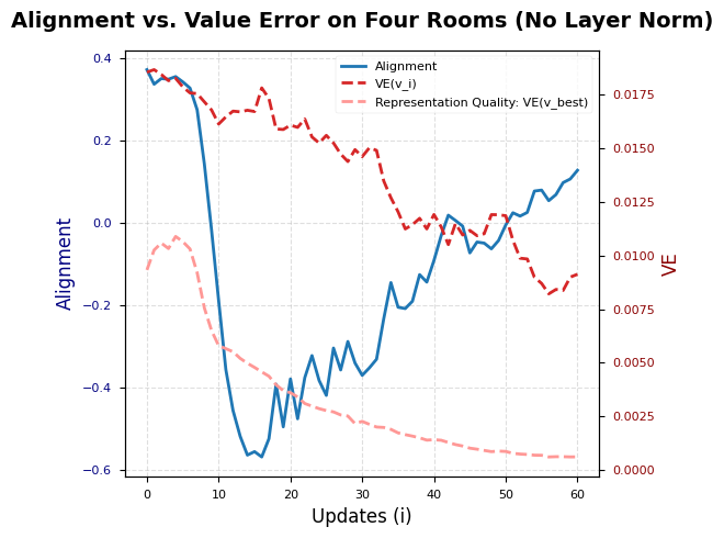
Figure 7: VE alignment during learning with no layer norm.

Wu et al 2025 showed that for the TD fixed point to exist, a condition they call rank invariance must hold: $\text{Rank}(\Phi) = \text{Rank}(\Phi^\top D(I-\gamma P) \Phi)$. They also showed that rank invariance is sufficient, in addition to being necessary for the TD fixed point to exist. ↩
Tsitsiklis, J.N. and Van Roy, B. An analysis of temporal-diﬀerence learning with function approximation. IEEE Transactions on Automatic Control,42(5):674–690, 1997 ↩
Scherrer, Bruno, Should one compute the Temporal Difference fix point or minimize the Bellman Residual? The unified oblique projection view, ICML 2010 ↩
Note that adding a layer norm after the output of the CNN was instrumental in achieving this very low value error. ↩