How reinforcement learning with TD learning depends on the inherent symmetry of the problem
(This is a follow-up to my previous post Will Deep TD Learning Result in Quality Representations?)
Deep temporal difference learning is the primary method for estimating the value function in reinforcement learning. The goal of TD learning is to minimize the average squared value error, averaged over a state distribution \(\mu\):
\[\overline{VE}(v, \mu) = \sum \mu(s) (V(s)-v(s))^2 = (V-v)^\intercal D (V-v)\]where \(V\) is the true value function, \(v\) is estimate, and \(D = \text{diag}[\mu]\). The value estimate, obtained from a neural network, is the dot product of the state-features and value weights: \(v(s) = \phi(s)^\intercal w\). Since the value is not directly observable, TD learning uses bootstrapping: fitting the value network towards a target based on its own predictions.
In the last post, I provided a geometric intuition and showed that deep TD learning can adjust the features in the wrong direction – raising the inherent value error \(VE\) for the best weights. This happened when the TD target and true value function are on opposite sides of the feature space, which I call misalignment. An example is pictured below.
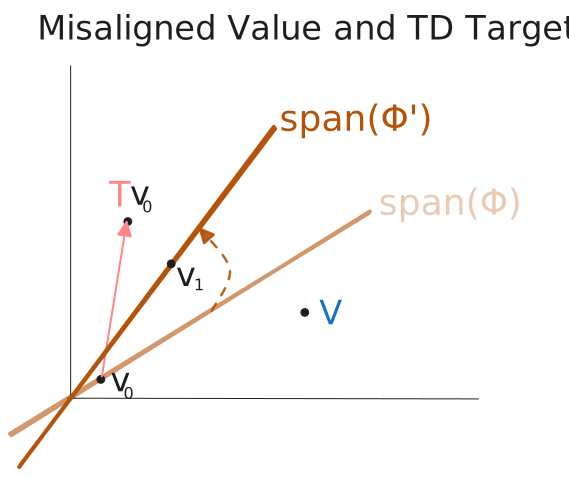
Figure 1: An example where misalignment of the bellman target Tv and true value function V hurts the features.
Is misalignment a problem in practice? For evaluating the random policy on Four Rooms, I found it was not. But does it become an issue in challenging domains like math or robotics?
The literature has explored how deep TD learning will adjust the features. [Tang and Munos 2023] showed that, under the property that the MDP is reversible (\(D P = P^\top D\)), the TD learning update happens to perform gradient descent on \(V\). This sounds great, however, reversibility is extremely unlikely to hold in practice: It says that the probability transition \(Ds_1 \rightarrow s_2\) equals the probability of \(s_2 \rightarrow s_1\). Yet, on most tasks, strong policies don’t go backwards.
In this post, I extend the results of Tang and Munos 2023. Reinforcing the importance of alignment, I show that alignment is a necessary and sufficient condition for the value error to decrease. I also show that an almost reversible property is enough to guarantee alignment. Before that, I walk us through their original proof, which answers the important question of when TD learning is doing the right thing. So let’s go!
Main Result of Tang and Munos (2023)
This work considers a continuous-time variant of TD learning, described by the following system of differential equations:
\[\begin{align} \dot{w}_t &= \eta_w \cdot \Phi_t^\top D(Tv_t - v_t)\\ \dot{\Phi}_t &= \eta_\Phi \cdot D(Tv_t-v_t) w^\top_t \end{align}\]The dot indicates the time derivative: (\(\dot{x}_t = \frac{dx}{dt}\) for a function \(x(t)\)). These equations describe the dynamics of TD learning when discrete algorithmic updates are brought into continuous time. For the purposes of this blog post, I’ll assume that the weights are a fixed value \(w_t = w\).
The key question is how the value error changes with each update. We analyze this in terms of the time-derivative of the value error, \(E\) (defined below).
We now define the value error. For theoretical convenience, Tang and Munos consider a loss that weights states slightly differently. They define a value error \(E\) that weights by the “key” matrix \(A = D(I-\gamma P)\):
\[\begin{align} E(\Phi, w) &\doteq \frac{1}{2} (\Phi w - V)^T A (\Phi w - V) \end{align}\]Though it doesn’t appear in the standard value error, the key matrix is of massive importance for the stability of TD learning. The dynamics of the features can be rewritten in terms of the key matrix.
\[\begin{align} \dot{\Phi}_t &= \eta_\Phi \cdot D(R + (I-\gamma P)v_t) w^\top\\ &= \eta_\Phi \cdot (DR + Av_t) w^\top \end{align}\]The true value function doesn’t appear directly. A key insight is that the Bellman equation implies \(DR = D(I-\gamma P) = AV\), allowing the above equation to be rewritten in terms of the true value function \(V\). This is an imporant move that is crucial to the results discussed in this post.
\[\begin{align} \dot{\Phi}_t &= -\eta_\Phi \cdot A(\Phi_t w-V) w^\top_t \end{align}\]We’d like to understand how \(E\) changes as TD learning progressively updates the features. Essentially this boils down to comparing \(\dot{\Phi}_t\) with \(-\partial_\Phi E(\Phi, w)\). If they point in the same direction, then TD learning decreases the value error.
Theorem (Tang and Munos 2023, Theorem 3): Assume that \(A\) is symmetric (i.e. \(DP = P^\top D\)). Then, the TD learning update is the same as gradient descent on \(E\), i.e.:
\[\dot{\Phi}_t \propto - \partial_{\Phi_t}E(\Phi_t).\]The conclusion is TD learning is effectively supervised learning of the value function. Sounds great! However, the premise that \(A\) is symmetric is unlikely to hold. It occurs when the Markov chain is reversible, meaning the probability of the transition \(s_1 \rightarrow s_2\) is the same as \(s_1 \leftarrow s_2\). Still, disregarding this result because the premise is too strong would be a mistake. As we will see, the proof of this theorem ties TD learning and value error minimization together in a way that can be extended, allowing us to write down exact mathematical conditions for when deep TD learning will and won’t work.
To start, I provide the proof of this theorem. Then I’ll relax the reversibility condition to show our main result.
Proof of Tang and Munos Theorem 3: Define the error vector \(e_t \doteq \Phi_t w - V^\pi\), which is a function of \(\Phi\). The value error is then: \(E(\Phi_t) = \frac{1}{2} e_t^T A e_t\) Since \(E\) is quadratic, it can be rewritten as \(e_t^\top (A + A^\top) e_t\), retaining only the symmetric portion of \(A\) (this is discussed more in the next section). From there, we have:
\[\begin{aligned} \partial_{\Phi_t} E &= \frac{1}{2} (A + A^\top) e_t w^\top\end{aligned}\]Now let’s consider the change in features due to TD learning. Plugging \(e_t\) into the expression \(\dot{\Phi}_t = -\eta_\Phi \cdot A(\Phi_i w_i-V) w^\top_i\) from earlier gives the following similar formula.
\[\begin{aligned} \dot{\Phi}_t &= -\eta_\Phi Ae_tw^\top\end{aligned}\]Comparing these formulations shows that if \(A\) is symmetric (\(A^\top = A\)), then TD learning gives the same feature update as gradient descent on \(E\).
New Result: When exactly do we have alignment?
For the TD learning update to be beneficial, we don’t need complete alignment of \(\dot{\Phi}_t\) and \(\partial_{\Phi_t} E\), only that \(\dot{E} < 0\). The chain rule gives \(\dot{E} = \langle \partial_\Phi E, \dot{\Phi} \rangle_F\) where \(\langle A, B\rangle_F \doteq \text{Tr}(A^\top B)\) is the Frobenius inner product. The takeaway is that \(E\) will decrease if \(\dot{\Phi}\) points in a direction of high alignment with \(-\partial_{\Phi_t} E\).
The main result of this post is the following, which says exactly when TD learning benefits the features.
\[\boxed{ \begin{align} \dot{E}(\Phi_t) < 0 \iff e_t^\top (A + A^\top ) A e_t > 0 \\ \end{align} }\]We can further simplify the inequality on the right. Let \(S\) and \(K\) denote the symmetric and skew-symmetric portions of \(A\). That is, \(A = S + K\) where \(S = \frac{1}{2}(A+ A^\top)\) and \(K = \frac{1}{2}(A- A^\top)\). Then, the inequality on the right is equivalent to:
\[\boxed{ \begin{aligned} e_t^\top S^2e_t > -\frac{1}{2}e_t^\top (SK - K S) e_t \end{aligned} }\]In other words, TD learning lowers the value error if and only if the key matrix \(A\) is symmetric enough, in the sense of the above equation.
Interpretation
How do we interpret the condition? Let’s first examine the terms of \(K\), and then connect this to the reversibility of the MDP.
The key matrix \(A = D(I-\gamma P)\) has off-diagonal terms like \(-\gamma \mu_i P_{ij}\). This leads to \(K\) having elements \(K_{ij} = \frac{\gamma }{2}(\mu_j P_{ji} - \mu_i P_{ij})\), which measure the extent to which the transition is non-reversible. When \(K_{ij}\) is zero, flow between the two states is equal (Tang and Munos’s theorem requires all elements of \(K\) are zero).
Intuitively, if the value error exists only in a region where the agent wanders back and forth equally, then TD learning will reduce \(E\) exactly like gradient descent.
However, in a one-way region, TD learning can raise \(E\) for certain values of \(e_t\). For example, an irreversible transition \(s_1 \rightarrow{} s_2\), where \(\phi(s_1)^\top \phi(s_2) \neq 0\) will see TD Learning update the features such that the value at \(s_1\) satisfies its own Bellman Equation, but it won’t take into account how changing these features affects the value of \(s_2\). This can create problems if \(v(s_2)\) is inaccurate. In contrast, gradient descent on \(E\) adjusts both \(\phi(s_1)\) and \(\phi(s_2)\).
Consider my previous experiment – evaluating the random policy on four rooms. It turns out that this is a highly symmetric Markov chain. Thus, it’s possible that my last example was inadvertently cherry-picked for TD learning to work. In an upcoming post, I’ll take a look at how easy it is to cherry pick highly non-reversible MDPs that make deep TD learning fail, even on-policy.
The resembelence of any such MDPs to practical problems may expose an area where we should be cautious using TD learning.
Proof of Main Result
To start the proof, apply the previously mentioned decomposition of \(A\) into symmetric and skew-symmetric parts.
\[\begin{align} A &= (1/2)(A + A^\top) + (1/2)(A - A^\top)\\ &= S + K \end{align}\]Note that for the skew-symmetric part \(K\), we have that \(u^\top K u=0\) for any vector \(u\).1 This yields:
\[E(\Phi_t, w) = e_t^\top S e_t\]From the symmetry of \(S\), we have the following expression for \(\dot{E}(\Phi_t)\).
\[\dot{E}(\Phi_t) = \frac{1}{2} \left(\dot{e}_t^\top S e_t + e_t S\dot{e}_t \right) = e_t^\top S \dot{e}_t = e_t^\top S \dot{\Phi}_t w\]To get this into the form of a Frobenius inner product, take the trace. For a scalar \(r\), \(\text{Tr}(r)=r\). Then apply the cyclic property of the trace: \(Tr(ABC) = Tr(CAB)\). Chaining these two together and then applying definition of the inner product, we get:
\[\begin{align} \dot{E}(\Phi_t) &= \text{Tr}(e_t^\top S \dot{\Phi}_t w) \\ &= \text{Tr}(w e_t^\top S \dot{\Phi}_t)\\ &= \langle S e_tw ^\top, \dot{\Phi}_t\rangle_F\\ &= \langle \partial_\Phi E, \dot{\Phi} \rangle_F \end{align}\]The last step follows since \(\partial_\Phi E$ = S e_t w^\top\), which can be seen from the first step of the Tang and Munos proof, or the chain rule definition of \(\dot{E}(\Phi_t)\). Notice that the improvement in \(E\) is synonymous with the following notion of alignment:
\[\text{Alignment} =-\langle \partial_\Phi E, \dot{\Phi}\rangle_F\]Next we determine when \(\dot{E}\) is negative (i.e. when alignment occurs). Starting from the trace expression above, and plugging in \(\dot{\Phi}_t = -\eta_\Phi A e_t w^\top\) allows us to pull out scalars:
\[\begin{align} \dot{E}(\Phi_t) &= - \eta_\Phi \cdot \text{Tr}\left(w e_t^\top S A e_t w^\top\right) \\ &= - \eta_\Phi \cdot \text{Tr}\left(w^\top w e_t^\top S A e_t \right) \\ &= - \eta_\Phi \cdot \|w \|_2^2 \cdot \text{Tr}\left(e_t^\top S A e_t \right) \\ \end{align}\]Since the scalar on the outside are negative, for the update to be beneficial, the argument to the trace must be positive. That is, the following guarantees alignment:
\[\boxed{ \begin{align} e_t^\top S A e_t > 0 \\ \end{align} }\]In other words, the TD learning update is guaranteed to help if the matrix \(SA = (A + A^\top)A\) is positive definite.2 Expanding the above expression:
\[\begin{align} e_t^\top S A e_t &= e_t^\top S (S+K) e_t \\ &= e_t^\top S^2e_t + e_t^\top SK e_t \\ \end{align}\]Next, apply symmetrization of \(SK = \frac{1}{2}(SK + S^\top K^\top) + \frac{1}{2}(SK - S^\top K^\top)\), the fact that \(K^\top = -K\), and the property of skew-symmetric matrices that \(v_t K v_t = 0\) for any vector \(v\).
\[\begin{align} &= e_t^\top S^2e_t + \frac{1}{2}e_t^\top (SK + K^\top S^\top) e_t + \frac{1}{2} e_t^\top (SK - K^\top S^\top) e_t \end{align}\] \[\begin{align} &= e_t^\top S^2e_t + \frac{1}{2}e_t^\top (SK - KS) e_t + \frac{1}{2} e_t^\top (SK + KS) e_t \\ &= e_t^\top \left( S^2 + \frac{1}{2} (SK - KS) \right) e_t \end{align}\]The last term is a quadratic with skew-symmetric weight (since \((SK + KS)^\top = -(KS-SK)\)), and is therefore \(0\). Also, we have that \(K^\top = -K\), which simplifies the second term. Re-arranging gives the final condition for when \(\dot{E}<0\), completing the proof.
\[\boxed{ \begin{aligned} e_t^\top S^2e_t > -\frac{1}{2}e_t^\top (SK - K S) e_t \end{aligned} }\]Note that the left hand side is always positive, since \(S\) is positive definite. The term on the right can be positive, negative, or zero, since \(SK-KS\) is indefinite (\(\text{Tr}(SK-KS)=Tr(SK)-Tr(KS)=0\)). This means that a beneficial update cannot be guaranteed for all error vectors \(e_t\), unless the symmetric portion of \(A\) dominates its skew-symmetric portion in the sense of the above equation.
Thanks for reading!